Extract summary from naivedensityraito object, including two-sample significance test for homogeneity of the numerator and denominator samples

Extract summary from naivedensityraito object, including two-sample significance test for homogeneity of the numerator and denominator samples

Usage

# S3 method for class 'naivedensityratio'
summary(
  object,
  test = FALSE,
  n_perm = 100,
  parallel = FALSE,
  cluster = NULL,
  ...
)

Arguments

object

Object of class naivedensityratio

test

logical indicating whether to statistically test for homogeneity of the numerator and denominator samples.

n_perm

Scalar indicating number of permutation samples

parallel

logical indicating to run the permutation test in parallel

cluster

NULL or a cluster object created by makeCluster. If NULL and parallel = TRUE, it uses the number of available cores minus 1.

...

further arguments passed to or from other methods.

Value

Summary of the fitted density ratio model

Examples

set.seed(123)
# Fit model
dr <- naive(numerator_small, denominator_small)
# Inspect model object
dr
#> 
#> Call:
#> naive(df_numerator = numerator_small, df_denominator = denominator_small)
#> 
#> Naive density ratio
#>   Number of variables: 3
#>   Number of numerator samples: 50
#>   Number of denominator samples: 100
#>   Numerator density: num [1:50] 1.41 5.74 1.87 4.13 1.67 ...
#>   Denominator density: num [1:100] 2.93 0.071 1.065 1.59 2.115 ...
#>  
# Obtain summary of model object
summary(dr)
#> 
#> Call:
#> naive(df_numerator = numerator_small, df_denominator = denominator_small)
#> 
#> Naive density ratio estimate:
#>   Number of variables: 
#>   Number of numerator samples: 50
#>   Number of denominator samples: 100
#>   Density ratio for numerator samples: num [1:50] 0.344 1.747 0.628 1.419 0.511 ...
#>   Density ratio for denominator samples: num [1:100] 1.0751 -2.6454 0.0626 0.464 0.7493 ...
#>  
#> 
#> Squared average log density ratio difference for numerator and denominator samples (SALDRD): 13.56
#> For a two-sample homogeneity test, use 'summary(x, test = TRUE)'.
#> 
# Plot model object
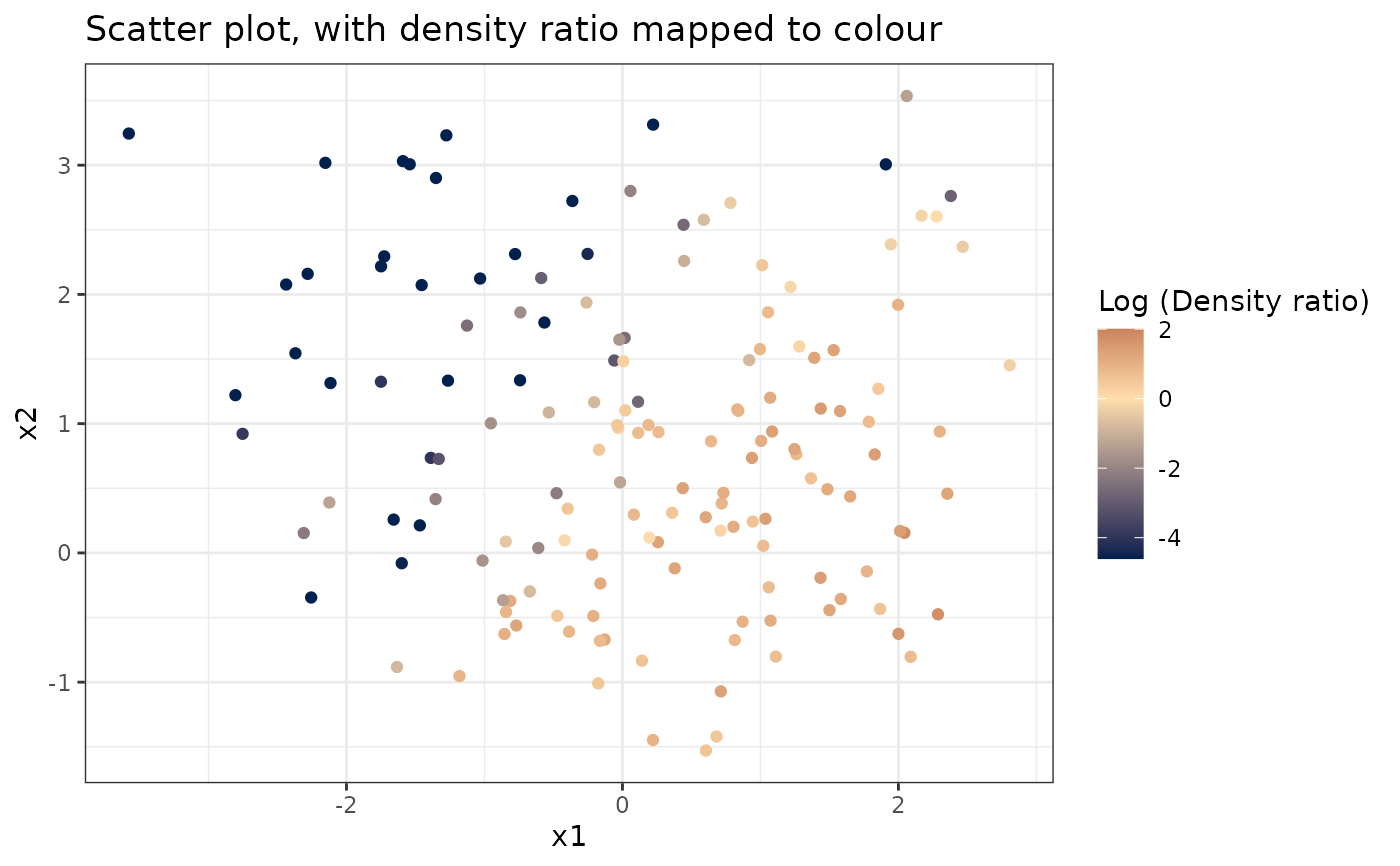
plot(dr)
#> Warning: Negative estimated density ratios for 25 observation(s) converted to 0.01 before applying logarithmic transformation
#> `stat_bin()` using `bins = 30`. Pick better value with `binwidth`.

# Plot density ratio for each variable individually
plot_univariate(dr)
#> Warning: Negative estimated density ratios for 25 observation(s) converted to 0.01 before applying logarithmic transformation
#> [[1]]

#> 
#> [[2]]

#> 
#> [[3]]

#> 
# Plot density ratio for each pair of variables
plot_bivariate(dr)
#> Warning: Negative estimated density ratios for 25 observation(s) converted to 0.01 before applying logarithmic transformation
#> [[1]]

#> 
#> [[2]]

#> 
#> [[3]]

#> 
# Predict density ratio and inspect first 6 predictions
head(predict(dr))
#> [1] 1.410607 5.739287 1.874031 4.131255 1.666760 4.095855
# Fit model with custom parameters
naive(numerator_small, denominator_small, m=2, kernel="epanechnikov")
#> 
#> Call:
#> naive(df_numerator = numerator_small, df_denominator = denominator_small,     m = 2, kernel = "epanechnikov")
#> 
#> Naive density ratio
#>   Number of variables: 3
#>   Number of numerator samples: 50
#>   Number of denominator samples: 100
#>   Numerator density: num [1:50] 0.572 1.421 0.945 1.058 0.936 ...
#>   Denominator density: num [1:100] 1.391 1.459 0.572 0.943 1.314 ...
#>