The naive approach creates separate kernel density estimates for
the numerator and the denominator samples, and then evaluates their
ratio for the denominator samples. For multivariate data, the density ratio
is computed after a orthogonal linear transformation, such that the new
variables can be treated as independent. To reduce the dimensionality of
the PCA solution, one can set the number of components by setting the
m parameter to an integer value smaller than the number of variables.
Usage
naive(
  df_numerator,
  df_denominator,
  m = NULL,
  bw = "SJ",
  kernel = "gaussian",
  n = 2L^11,
  ...
)
Arguments
- df_numerator
data.framewith exclusively numeric variables with the numerator samples- df_denominator
data.framewith exclusively numeric variables with the denominator samples (must have the same variables asdf_denominator)- m
integerOptional parameter to reduce the dimensionality of the data in multivariate density ratio estimation problems. If missing, the number of variables in the data is used. If set to an integer value smaller than the number of variables, the firstmprincipal components are used to estimate the density ratio. If set toNULL, the square root of the number of variables is used (for consistency with other methods).- bw
the smoothing bandwidth to be used. See stats::density for more information.
- kernel
the kernel to be used. See stats::density for more information.
- n
integerthe number of equally spaced points at which the density is to be estimated. When n > 512, it is rounded up to a power of 2 during the calculations (as fast Fourier transform is used) and the final result is interpolated by stats::approx. So it makes sense to specify n as a power' of two.- ...
further arguments passed to stats::density
Examples
set.seed(123)
# Fit model
dr <- naive(numerator_small, denominator_small)
# Inspect model object
dr
#>
#> Call:
#> naive(df_numerator = numerator_small, df_denominator = denominator_small)
#>
#> Naive density ratio
#> Number of variables: 3
#> Number of numerator samples: 50
#> Number of denominator samples: 100
#> Numerator density: num [1:50] 1.41 5.74 1.87 4.13 1.67 ...
#> Denominator density: num [1:100] 2.93 0.071 1.065 1.59 2.115 ...
#>
# Obtain summary of model object
summary(dr)
#>
#> Call:
#> naive(df_numerator = numerator_small, df_denominator = denominator_small)
#>
#> Naive density ratio estimate:
#> Number of variables:
#> Number of numerator samples: 50
#> Number of denominator samples: 100
#> Density ratio for numerator samples: num [1:50] 0.344 1.747 0.628 1.419 0.511 ...
#> Density ratio for denominator samples: num [1:100] 1.0751 -2.6454 0.0626 0.464 0.7493 ...
#>
#>
#> Squared average log density ratio difference for numerator and denominator samples (SALDRD): 13.56
#> For a two-sample homogeneity test, use 'summary(x, test = TRUE)'.
#>
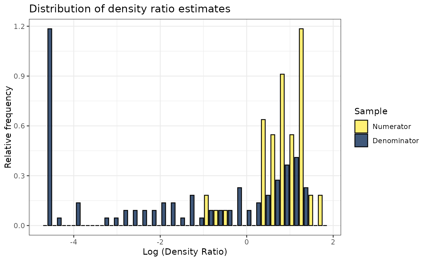
# Plot model object
plot(dr)
#> Warning: Negative estimated density ratios for 25 observation(s) converted to 0.01 before applying logarithmic transformation
#> `stat_bin()` using `bins = 30`. Pick better value `binwidth`.
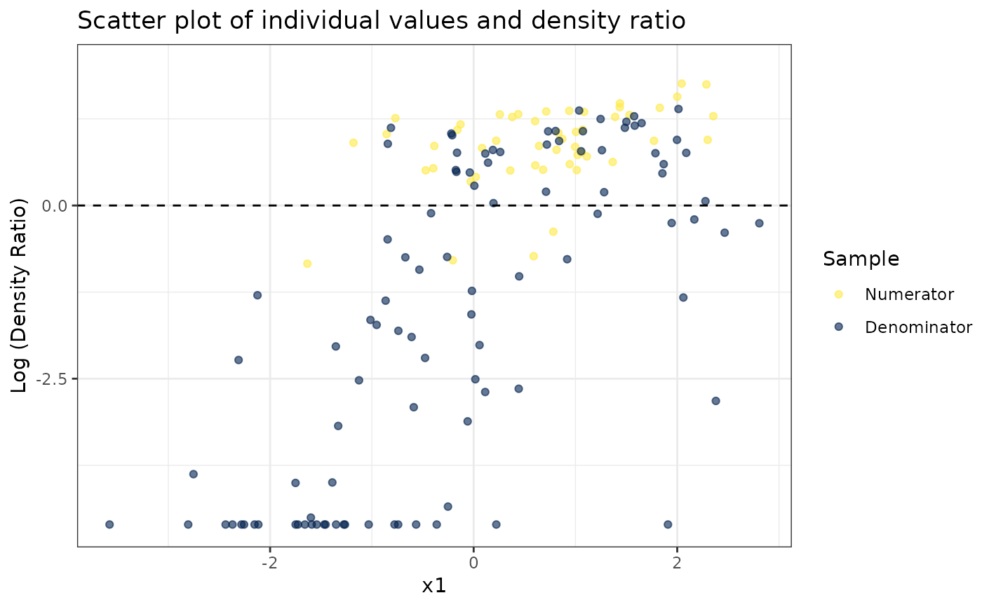
 # Plot density ratio for each variable individually
plot_univariate(dr)
#> Warning: Negative estimated density ratios for 25 observation(s) converted to 0.01 before applying logarithmic transformation
#> [[1]]
# Plot density ratio for each variable individually
plot_univariate(dr)
#> Warning: Negative estimated density ratios for 25 observation(s) converted to 0.01 before applying logarithmic transformation
#> [[1]]
 #>
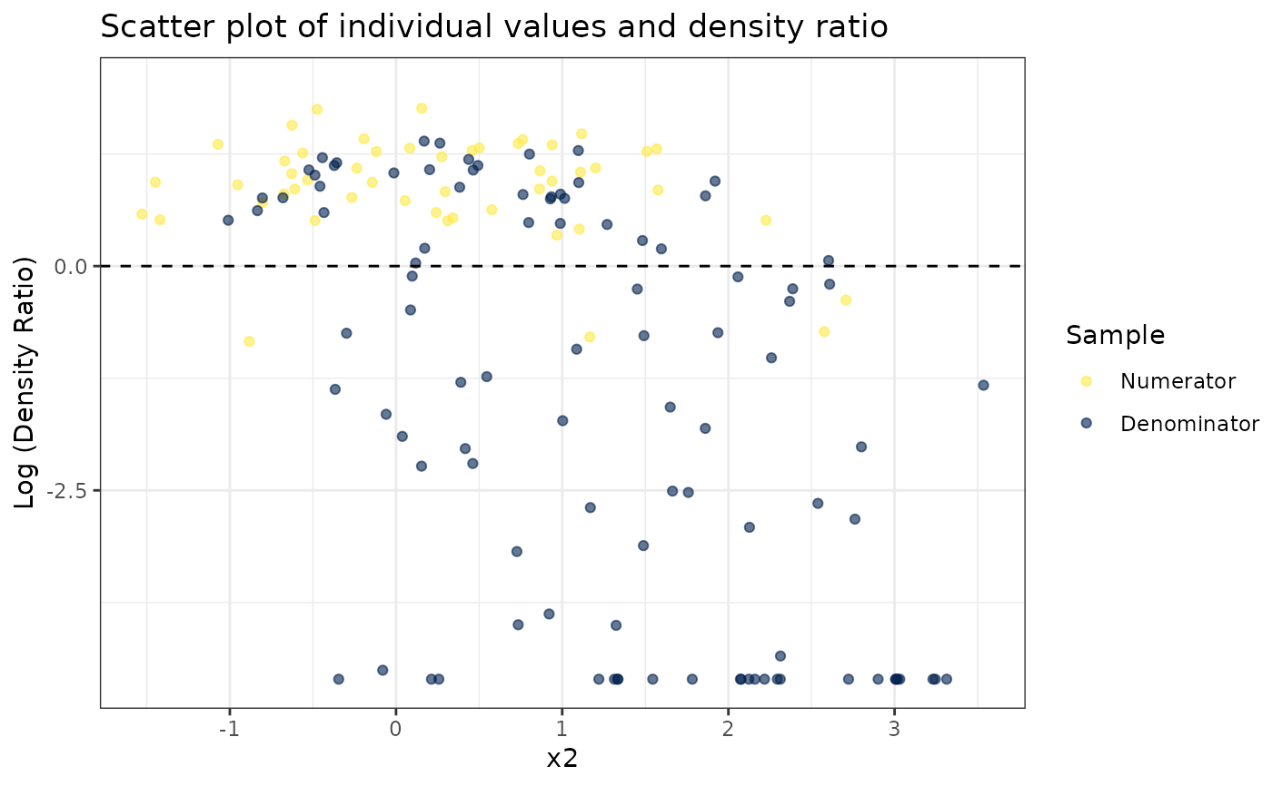
#> [[2]]
#>
#> [[2]]
 #>
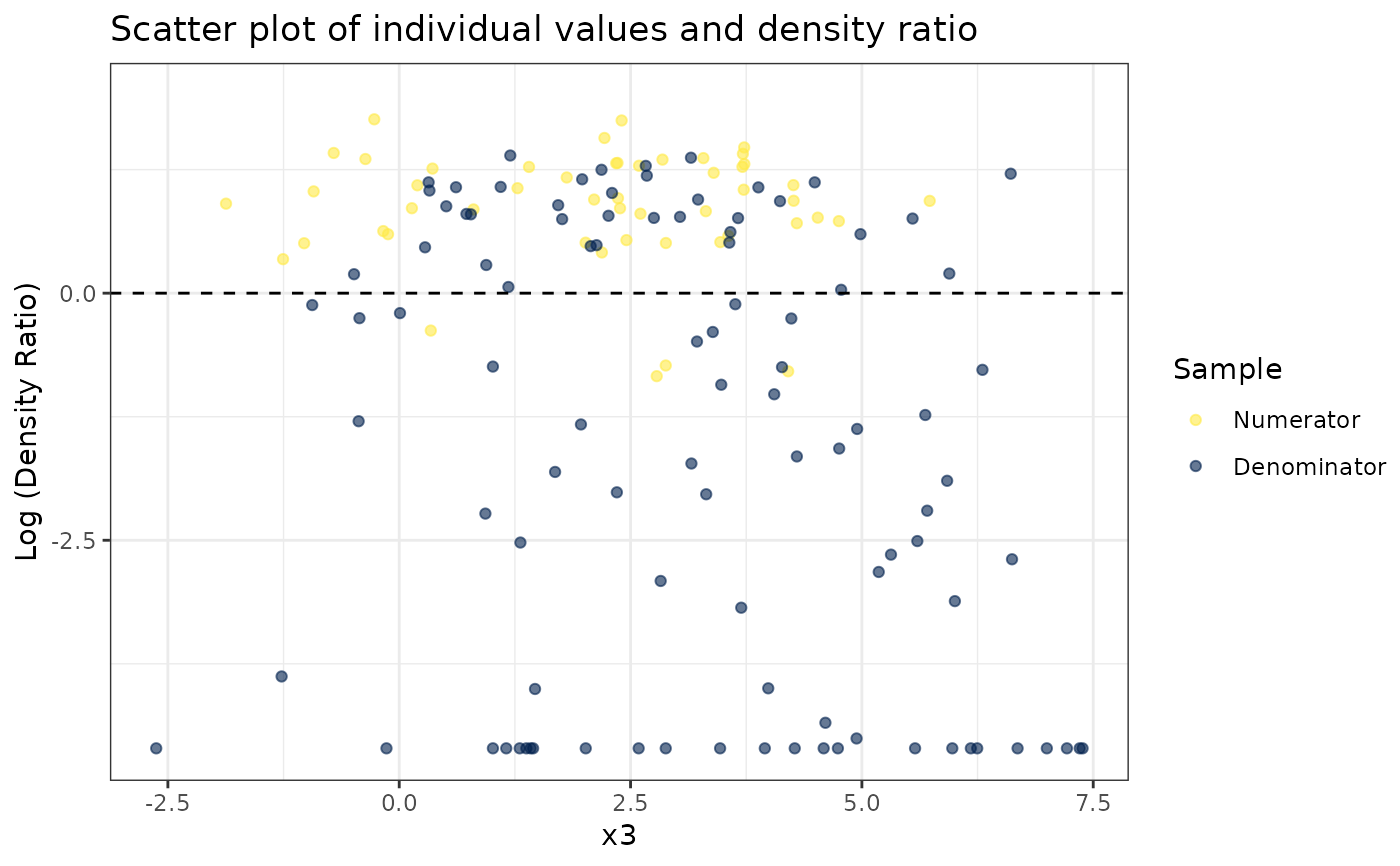
#> [[3]]
#>
#> [[3]]
 #>
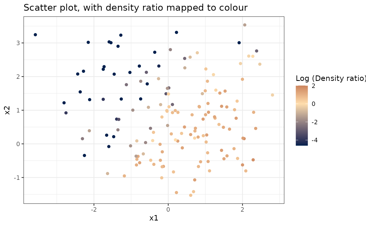
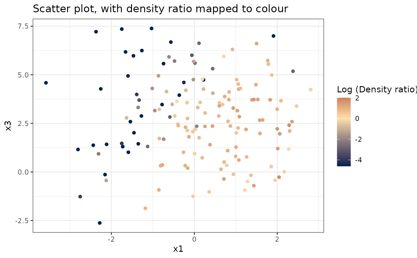
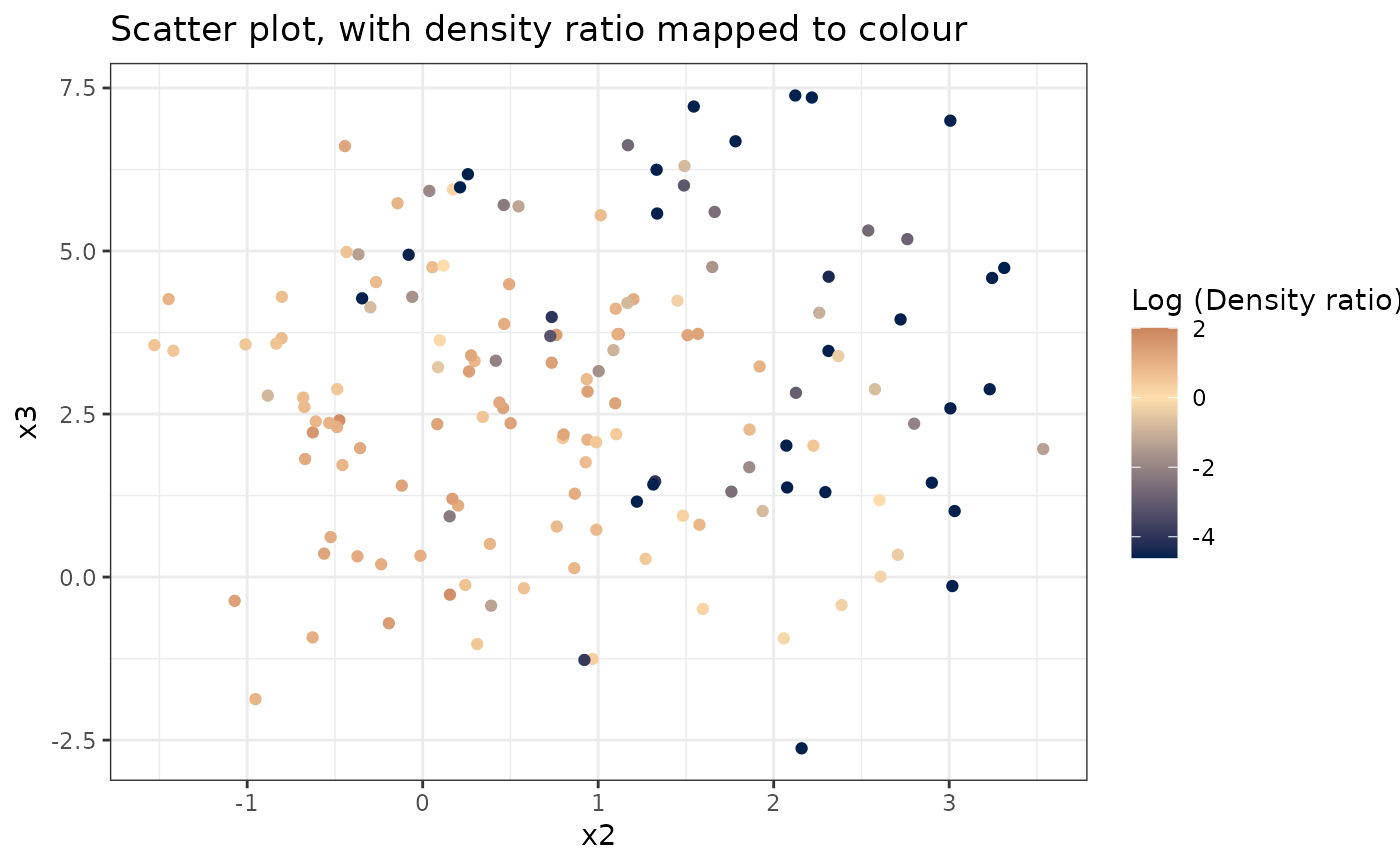
# Plot density ratio for each pair of variables
plot_bivariate(dr)
#> Warning: Negative estimated density ratios for 25 observation(s) converted to 0.01 before applying logarithmic transformation
#> [[1]]
#>
# Plot density ratio for each pair of variables
plot_bivariate(dr)
#> Warning: Negative estimated density ratios for 25 observation(s) converted to 0.01 before applying logarithmic transformation
#> [[1]]
 #>
#> [[2]]
#>
#> [[2]]
 #>
#> [[3]]
#>
#> [[3]]
 #>
# Predict density ratio and inspect first 6 predictions
head(predict(dr))
#> [1] 1.410607 5.739287 1.874031 4.131255 1.666760 4.095855
# Fit model with custom parameters
naive(numerator_small, denominator_small, m=2, kernel="epanechnikov")
#>
#> Call:
#> naive(df_numerator = numerator_small, df_denominator = denominator_small, m = 2, kernel = "epanechnikov")
#>
#> Naive density ratio
#> Number of variables: 3
#> Number of numerator samples: 50
#> Number of denominator samples: 100
#> Numerator density: num [1:50] 0.572 1.421 0.945 1.058 0.936 ...
#> Denominator density: num [1:100] 1.391 1.459 0.572 0.943 1.314 ...
#>
#>
# Predict density ratio and inspect first 6 predictions
head(predict(dr))
#> [1] 1.410607 5.739287 1.874031 4.131255 1.666760 4.095855
# Fit model with custom parameters
naive(numerator_small, denominator_small, m=2, kernel="epanechnikov")
#>
#> Call:
#> naive(df_numerator = numerator_small, df_denominator = denominator_small, m = 2, kernel = "epanechnikov")
#>
#> Naive density ratio
#> Number of variables: 3
#> Number of numerator samples: 50
#> Number of denominator samples: 100
#> Numerator density: num [1:50] 0.572 1.421 0.945 1.058 0.936 ...
#> Denominator density: num [1:100] 1.391 1.459 0.572 0.943 1.314 ...
#>