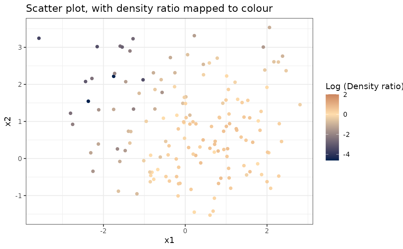
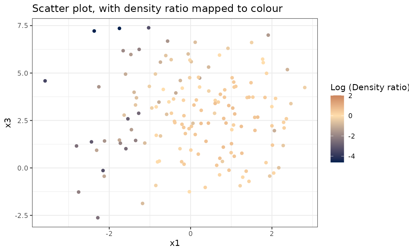
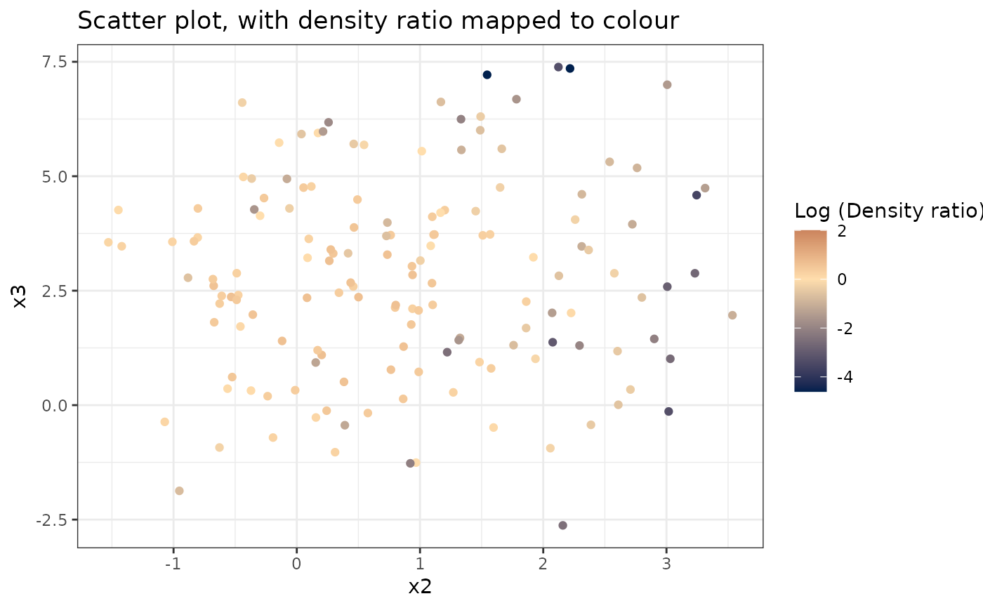
Plots a scatterplot of two variables, with densityratio mapped to the colour scale.
Usage
plot_bivariate(
  x,
  vars = NULL,
  samples = "both",
  grid = FALSE,
  logscale = TRUE,
  show.sample = FALSE,
  tol = 0.01,
  ...
)
Arguments
- x
Density ratio object created with e.g.,
kliep(),ulsif(), ornaive()- vars
Character vector of variable names for which all pairwise bivariate plots are created
- samples
Character string indicating whether to plot the 'numerator', 'denominator', or 'both' samples. Default is 'both'.
- grid
Logical indicating whether output should be a list of individual plots ("individual"), or one facetted plot with all variables ("assembled"). Defaults to "individual".
- logscale
Logical indicating whether to plot the density ratio estimates on a log scale. Default is
TRUE.- show.sample
Logical indicating whether to give different shapes to observations, depending on the sample they come from (numerator or denominator). Defaults to
FALSE.- tol
Numeric indicating the tolerance: values below this value will be set to the tolerance value, for legibility of the plots
- ...
Additional arguments passed to the predict() function.
Examples
set.seed(123)
# Fit model
dr <- ulsif(numerator_small, denominator_small)
# Inspect model object
dr
#>
#> Call:
#> ulsif(df_numerator = numerator_small, df_denominator = denominator_small)
#>
#> Kernel Information:
#> Kernel type: Gaussian with L2 norm distances
#> Number of kernels: 150
#> sigma: num [1:10] 0.711 1.08 1.333 1.538 1.742 ...
#>
#> Regularization parameter (lambda): num [1:20] 1000 483.3 233.6 112.9 54.6 ...
#>
#> Optimal sigma (loocv): 3.425852
#> Optimal lambda (loocv): 0.6951928
#> Optimal kernel weights (loocv): num [1:150] 0.05072 0.09115 0.07853 0.10771 -0.00969 ...
#>
# Obtain summary of model object
summary(dr)
#>
#> Call:
#> ulsif(df_numerator = numerator_small, df_denominator = denominator_small)
#>
#> Kernel Information:
#> Kernel type: Gaussian with L2 norm distances
#> Number of kernels: 150
#>
#> Optimal sigma: 3.425852
#> Optimal lambda: 0.6951928
#> Optimal kernel weights: num [1:150] 0.05072 0.09115 0.07853 0.10771 -0.00969 ...
#>
#> Pearson divergence between P(nu) and P(de): 0.3872
#> For a two-sample homogeneity test, use 'summary(x, test = TRUE)'.
#>
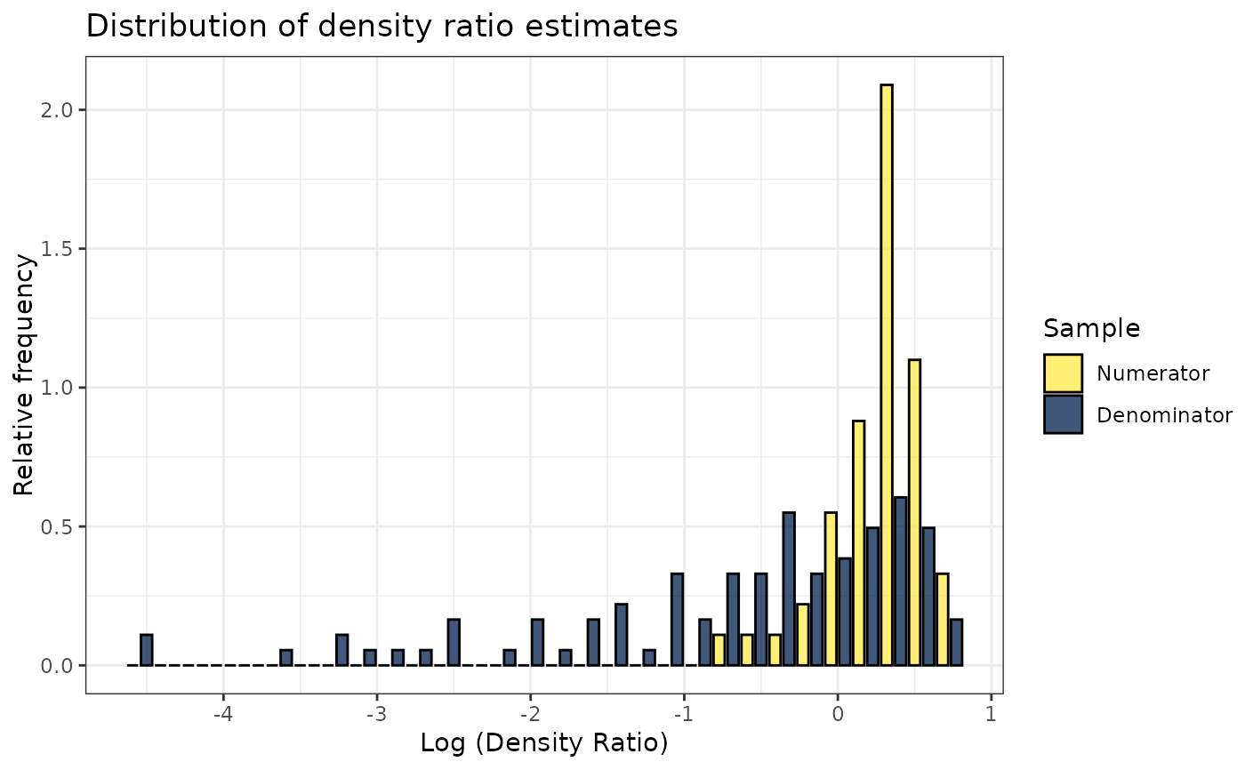
# Plot model object
plot(dr)
#> Warning: Negative estimated density ratios for 7 observation(s) converted to 0.01 before applying logarithmic transformation
#> `stat_bin()` using `bins = 30`. Pick better value `binwidth`.
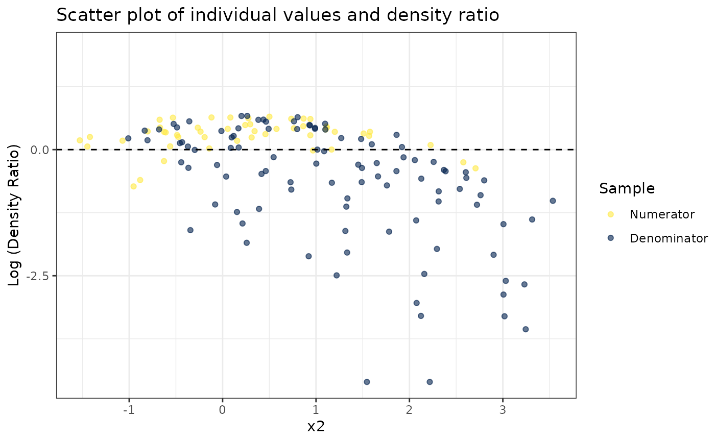
 # Plot density ratio for each variable individually
plot_univariate(dr)
#> Warning: Negative estimated density ratios for 7 observation(s) converted to 0.01 before applying logarithmic transformation
#> [[1]]
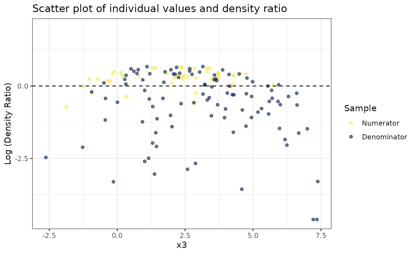
# Plot density ratio for each variable individually
plot_univariate(dr)
#> Warning: Negative estimated density ratios for 7 observation(s) converted to 0.01 before applying logarithmic transformation
#> [[1]]
 #>
#> [[2]]
#>
#> [[2]]
 #>
#> [[3]]
#>
#> [[3]]
 #>
# Plot density ratio for each pair of variables
plot_bivariate(dr)
#> Warning: Negative estimated density ratios for 7 observation(s) converted to 0.01 before applying logarithmic transformation
#> [[1]]
#>
# Plot density ratio for each pair of variables
plot_bivariate(dr)
#> Warning: Negative estimated density ratios for 7 observation(s) converted to 0.01 before applying logarithmic transformation
#> [[1]]
 #>
#> [[2]]
#>
#> [[2]]
 #>
#> [[3]]
#>
#> [[3]]
 #>
# Predict density ratio and inspect first 6 predictions
head(predict(dr))
#> , , 1
#>
#> [,1]
#> [1,] 1.637268
#> [2,] 2.230380
#> [3,] 2.147449
#> [4,] 2.302901
#> [5,] 1.228723
#> [6,] 1.785768
#>
# Fit model with custom parameters
ulsif(numerator_small, denominator_small, sigma = 2, lambda = 2)
#>
#> Call:
#> ulsif(df_numerator = numerator_small, df_denominator = denominator_small, sigma = 2, lambda = 2)
#>
#> Kernel Information:
#> Kernel type: Gaussian with L2 norm distances
#> Number of kernels: 150
#> sigma: num 2
#>
#> Regularization parameter (lambda): num 2
#>
#> Optimal sigma (loocv): 2
#> Optimal lambda (loocv): 2
#> Optimal kernel weights (loocv): num [1:150] 0.0353 0.0558 0.0534 0.0622 0.0111 ...
#>
#>
# Predict density ratio and inspect first 6 predictions
head(predict(dr))
#> , , 1
#>
#> [,1]
#> [1,] 1.637268
#> [2,] 2.230380
#> [3,] 2.147449
#> [4,] 2.302901
#> [5,] 1.228723
#> [6,] 1.785768
#>
# Fit model with custom parameters
ulsif(numerator_small, denominator_small, sigma = 2, lambda = 2)
#>
#> Call:
#> ulsif(df_numerator = numerator_small, df_denominator = denominator_small, sigma = 2, lambda = 2)
#>
#> Kernel Information:
#> Kernel type: Gaussian with L2 norm distances
#> Number of kernels: 150
#> sigma: num 2
#>
#> Regularization parameter (lambda): num 2
#>
#> Optimal sigma (loocv): 2
#> Optimal lambda (loocv): 2
#> Optimal kernel weights (loocv): num [1:150] 0.0353 0.0558 0.0534 0.0622 0.0111 ...
#>