Extract summary from lhss object, including two-sample significance test for homogeneity of the numerator and denominator samples
Source: R/summary.R
summary.lhss.RdExtract summary from lhss object, including two-sample significance
test for homogeneity of the numerator and denominator samples
Usage
# S3 method for class 'lhss'
summary(
  object,
  test = FALSE,
  n_perm = 100,
  parallel = FALSE,
  cluster = NULL,
  ...
)
Arguments
- object
Object of class
lhss- test
logical indicating whether to statistically test for homogeneity of the numerator and denominator samples.
- n_perm
Scalar indicating number of permutation samples
- parallel
logicalindicating to run the permutation test in parallel- cluster
NULLor a cluster object created bymakeCluster. IfNULLandparallel = TRUE, it uses the number of available cores minus 1.- ...
further arguments passed to or from other methods.
Examples
set.seed(123)
# Fit model (minimal example to limit computation time)
dr <- lhss(numerator_small, denominator_small,
nsigma = 3, lambda = c(0.1, 1), ncenters = 50, maxit = 100)
# Inspect model object
dr
#>
#> Call:
#> lhss(df_numerator = numerator_small, df_denominator = denominator_small, nsigma = 3, lambda = c(0.1, 1), ncenters = 50, maxit = 100)
#>
#> Kernel Information:
#> Kernel type: Gaussian with L2 norm distances
#> Number of kernels: 50
#> sigma: num [1:3, 1:2] 0.0793 0.9371 2.677 0.0693 0.9633 ...
#>
#> Regularization parameter (lambda): num [1:2] 0.1 1
#>
#> Subspace dimension (m): 1
#> Optimal sigma: 2.677003
#> Optimal lambda: 0.1
#> Optimal kernel weights (loocv): num [1:51] 6.666 -0.3081 -0.0385 -0.0353 0.0108 ...
#>
# Obtain summary of model object
summary(dr)
#>
#> Call:
#> lhss(df_numerator = numerator_small, df_denominator = denominator_small, nsigma = 3, lambda = c(0.1, 1), ncenters = 50, maxit = 100)
#>
#> Kernel Information:
#> Kernel type: Gaussian with L2 norm distances
#> Number of kernels: 50
#>
#> Subspace dimension (m): 1
#> Optimal sigma: 2.677003
#> Optimal lambda: 0.1
#> Optimal kernel weights (loocv): num [1:51] 6.666 -0.3081 -0.0385 -0.0353 0.0108 ...
#>
#> Pearson divergence between P(nu) and P(de): 0.6358
#> For a two-sample homogeneity test, use 'summary(x, test = TRUE)'.
#>
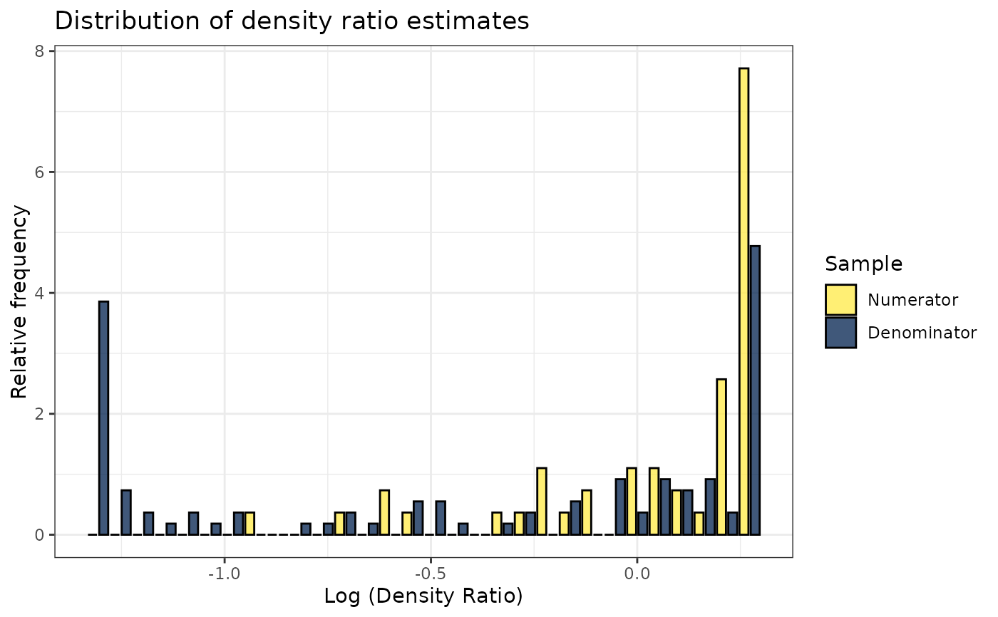
# Plot model object
plot(dr)
#> Warning: Negative estimated density ratios for 12 observation(s) converted to 0.01 before applying logarithmic transformation
#> `stat_bin()` using `bins = 30`. Pick better value `binwidth`.
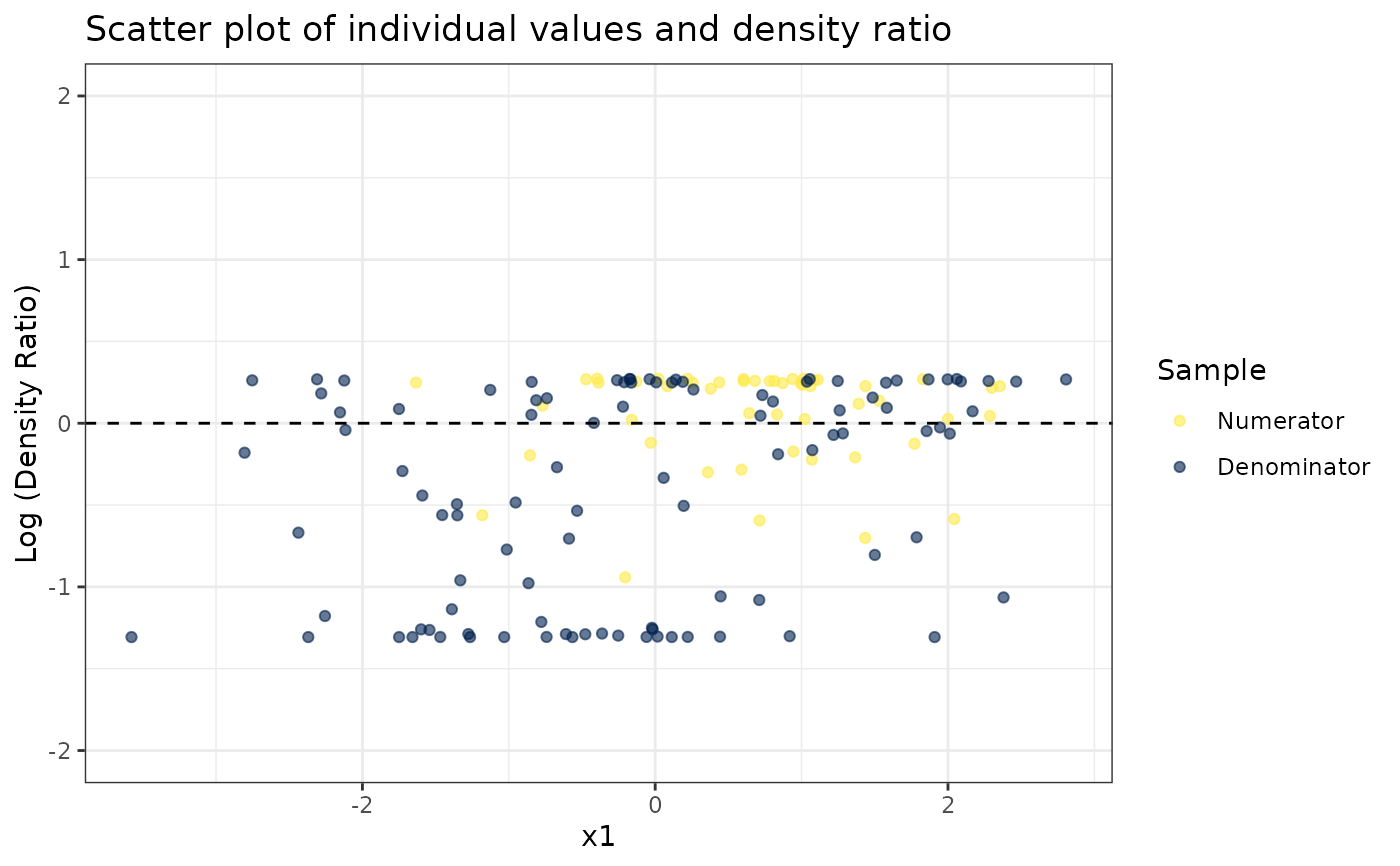
 # Plot density ratio for each variable individually
plot_univariate(dr)
#> Warning: Negative estimated density ratios for 12 observation(s) converted to 0.01 before applying logarithmic transformation
#> [[1]]
# Plot density ratio for each variable individually
plot_univariate(dr)
#> Warning: Negative estimated density ratios for 12 observation(s) converted to 0.01 before applying logarithmic transformation
#> [[1]]
 #>
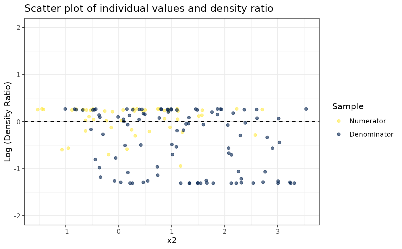
#> [[2]]
#>
#> [[2]]
 #>
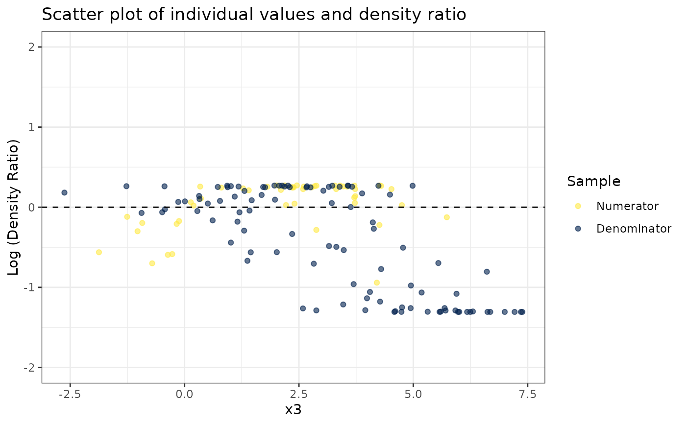
#> [[3]]
#>
#> [[3]]
 #>
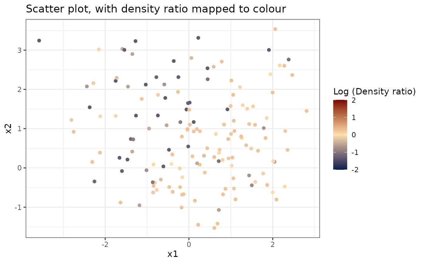
# Plot density ratio for each pair of variables
plot_bivariate(dr)
#> Warning: Negative estimated density ratios for 12 observation(s) converted to 0.01 before applying logarithmic transformation
#> [[1]]
#>
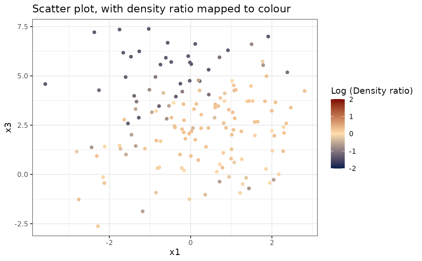
# Plot density ratio for each pair of variables
plot_bivariate(dr)
#> Warning: Negative estimated density ratios for 12 observation(s) converted to 0.01 before applying logarithmic transformation
#> [[1]]
 #>
#> [[2]]
#>
#> [[2]]
 #>
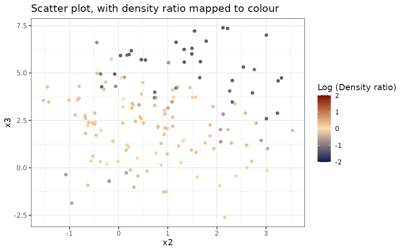
#> [[3]]
#>
#> [[3]]
 #>
# Predict density ratio and inspect first 6 predictions
head(predict(dr))
#> , , 1
#>
#> [,1]
#> [1,] 2.1625009
#> [2,] 3.6694722
#> [3,] 2.7969688
#> [4,] 4.1387638
#> [5,] 0.1585054
#> [6,] 1.2616673
#>
#>
# Predict density ratio and inspect first 6 predictions
head(predict(dr))
#> , , 1
#>
#> [,1]
#> [1,] 2.1625009
#> [2,] 3.6694722
#> [3,] 2.7969688
#> [4,] 4.1387638
#> [5,] 0.1585054
#> [6,] 1.2616673
#>