Least-squares heterodistributional subspace search
Usage
lhss(
  df_numerator,
  df_denominator,
  m = NULL,
  intercept = TRUE,
  scale = "numerator",
  nsigma = 10,
  sigma_quantile = NULL,
  sigma = NULL,
  nlambda = 10,
  lambda = NULL,
  ncenters = 200,
  centers = NULL,
  maxit = 200,
  progressbar = TRUE
)
Arguments
- df_numerator
data.framewith exclusively numeric variables with the numerator samples- df_denominator
data.framewith exclusively numeric variables with the denominator samples (must have the same variables asdf_denominator)- m
Scalar indicating the dimensionality of the reduced subspace
- intercept
logicalIndicating whether to include an intercept term in the model. Defaults toTRUE.- scale
"numerator","denominator", orNULL, indicating whether to standardize each numeric variable according to the numerator means and standard deviations, the denominator means and standard deviations, or apply no standardization at all.- nsigma
Integer indicating the number of sigma values (bandwidth parameter of the Gaussian kernel gram matrix) to use in cross-validation.
- sigma_quantile
NULLor numeric vector with probabilities to calculate the quantiles of the distance matrix to obtain sigma values. IfNULL,nsigmavalues between0.05and0.95are used.- sigma
NULLor a scalar value to determine the bandwidth of the Gaussian kernel gram matrix. IfNULL,nsigmavalues between0.05and0.95are used.- nlambda
Integer indicating the number of
lambdavalues (regularization parameter), by default,lambdais set to10^seq(3, -3, length.out = nlambda).- lambda
NULLor numeric vector indicating the lambda values to use in cross-validation- ncenters
integerMaximum number of Gaussian centers in the kernel gram matrix.- centers
NULLordata.framewith the same dimensions as the data, indicating the centers for the Gaussian kernel gram matrix.- maxit
Maximum number of iterations in the updating scheme.
- progressbar
Logical indicating whether or not to display a progressbar.
Value
lhss-object, containing all information to calculate the
density ratio using optimal sigma, optimal lambda and optimal weights.
References
Sugiyama, M., Yamada, M., Von Bünau, P., Suzuki, T., Kanamori, T. & Kawanabe, M. (2011). Direct density-ratio estimation with dimensionality reduction via least-squares hetero-distributional subspace search. Neural Networks, 24, 183-198. doi:10.1016/j.neunet.2010.10.005 .
Examples
set.seed(123)
# Fit model (minimal example to limit computation time)
dr <- lhss(numerator_small, denominator_small,
nsigma = 3, lambda = c(0.1, 1), ncenters = 50, maxit = 100)
# Inspect model object
dr
#>
#> Call:
#> lhss(df_numerator = numerator_small, df_denominator = denominator_small, nsigma = 3, lambda = c(0.1, 1), ncenters = 50, maxit = 100)
#>
#> Kernel Information:
#> Kernel type: Gaussian with L2 norm distances
#> Number of kernels: 50
#> sigma: num [1:3, 1:2] 0.0793 0.9371 2.677 0.0693 0.9633 ...
#>
#> Regularization parameter (lambda): num [1:2] 0.1 1
#>
#> Subspace dimension (m): 1
#> Optimal sigma: 2.677003
#> Optimal lambda: 0.1
#> Optimal kernel weights (loocv): num [1:51] 6.666 -0.3081 -0.0385 -0.0353 0.0108 ...
#>
# Obtain summary of model object
summary(dr)
#>
#> Call:
#> lhss(df_numerator = numerator_small, df_denominator = denominator_small, nsigma = 3, lambda = c(0.1, 1), ncenters = 50, maxit = 100)
#>
#> Kernel Information:
#> Kernel type: Gaussian with L2 norm distances
#> Number of kernels: 50
#>
#> Subspace dimension (m): 1
#> Optimal sigma: 2.677003
#> Optimal lambda: 0.1
#> Optimal kernel weights (loocv): num [1:51] 6.666 -0.3081 -0.0385 -0.0353 0.0108 ...
#>
#> Pearson divergence between P(nu) and P(de): 0.6358
#> For a two-sample homogeneity test, use 'summary(x, test = TRUE)'.
#>
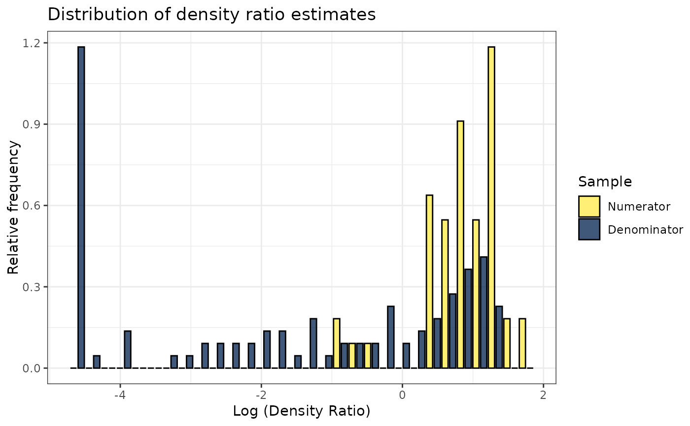
# Plot model object
plot(dr)
#> Warning: Negative estimated density ratios for 12 observation(s) converted to 0.01 before applying logarithmic transformation
#> `stat_bin()` using `bins = 30`. Pick better value `binwidth`.
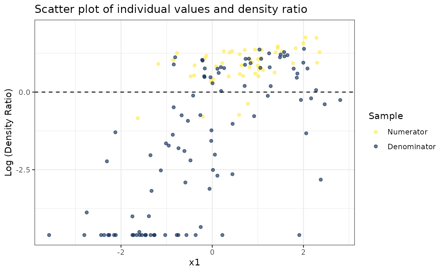
 # Plot density ratio for each variable individually
plot_univariate(dr)
#> Warning: Negative estimated density ratios for 12 observation(s) converted to 0.01 before applying logarithmic transformation
#> [[1]]
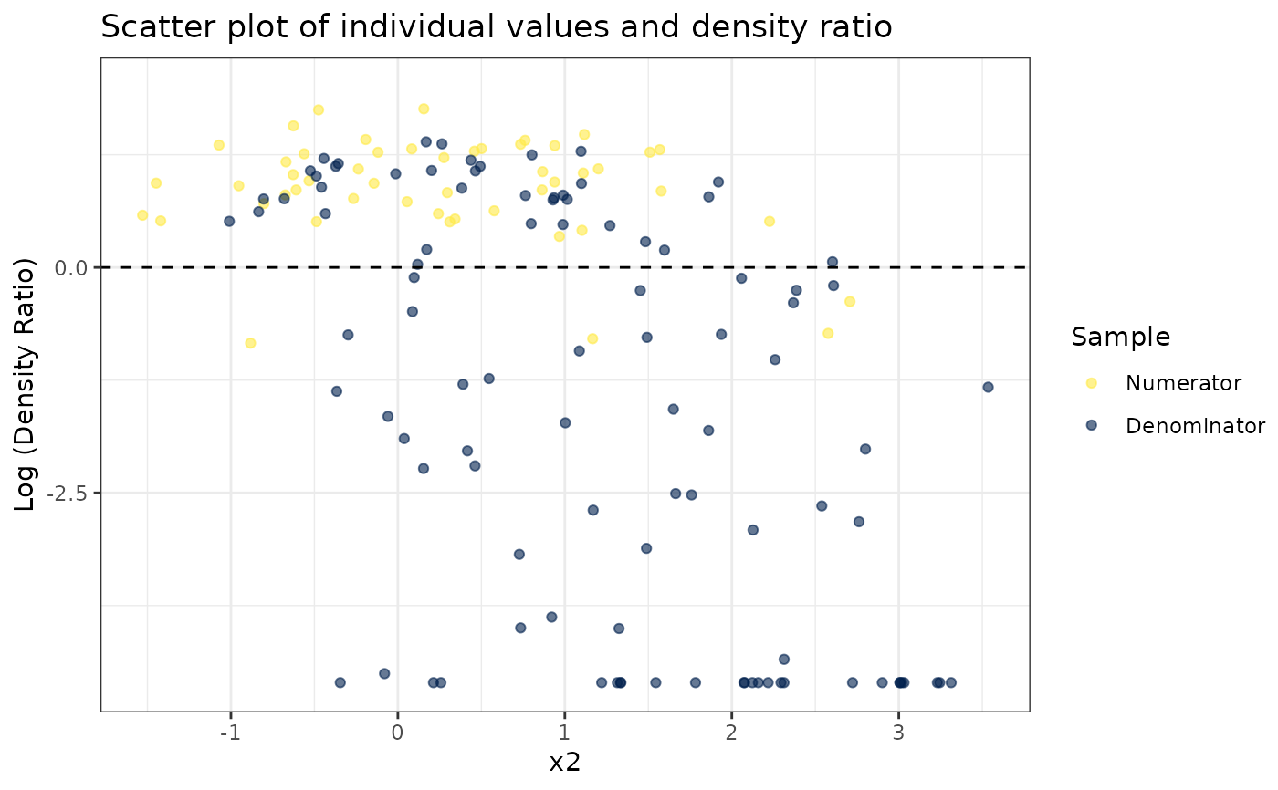
# Plot density ratio for each variable individually
plot_univariate(dr)
#> Warning: Negative estimated density ratios for 12 observation(s) converted to 0.01 before applying logarithmic transformation
#> [[1]]
 #>
#> [[2]]
#>
#> [[2]]
 #>
#> [[3]]
#>
#> [[3]]
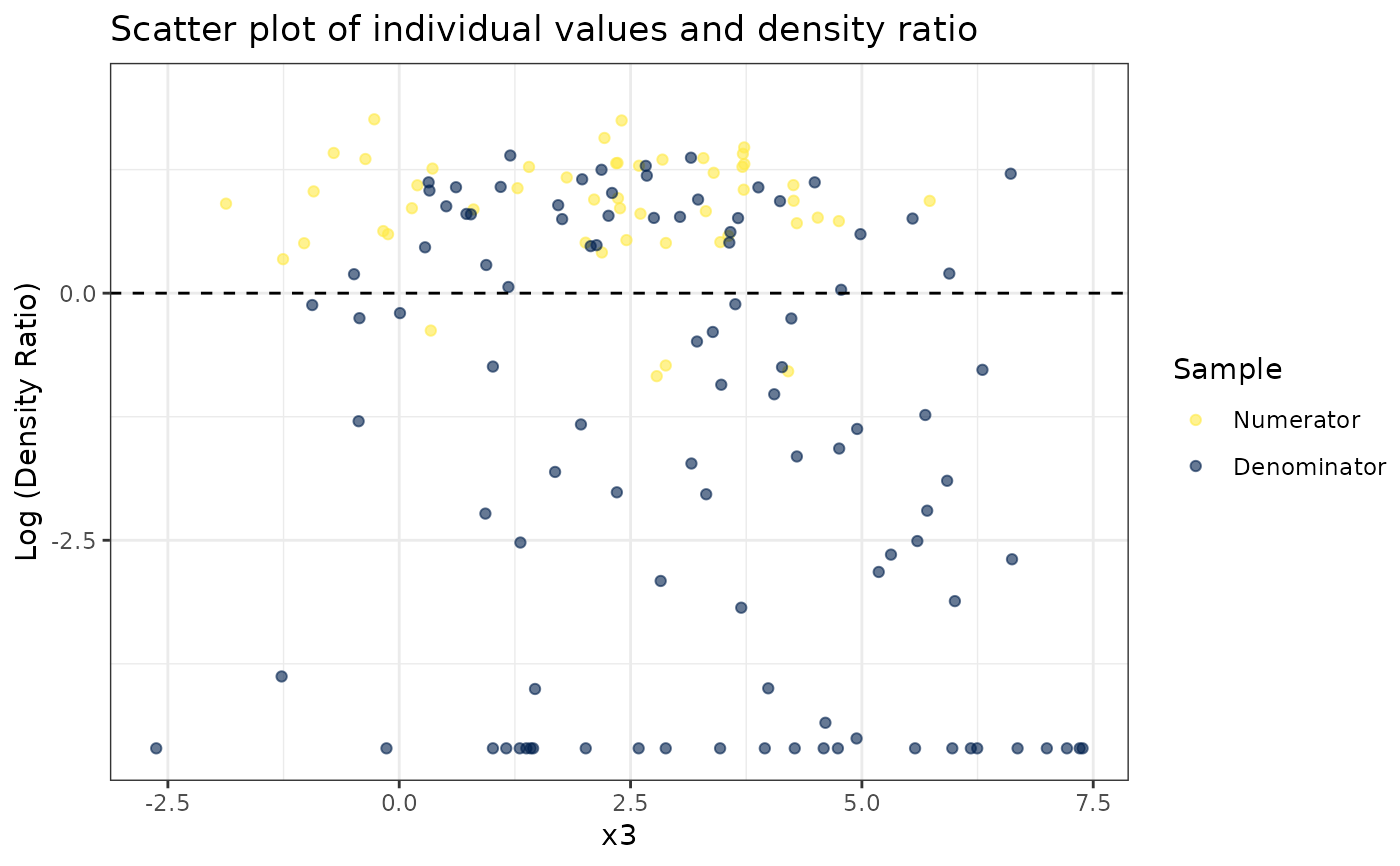 #>
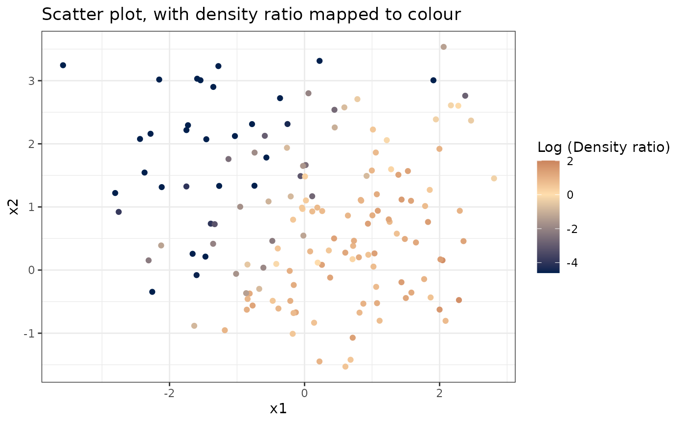
# Plot density ratio for each pair of variables
plot_bivariate(dr)
#> Warning: Negative estimated density ratios for 12 observation(s) converted to 0.01 before applying logarithmic transformation
#> [[1]]
#>
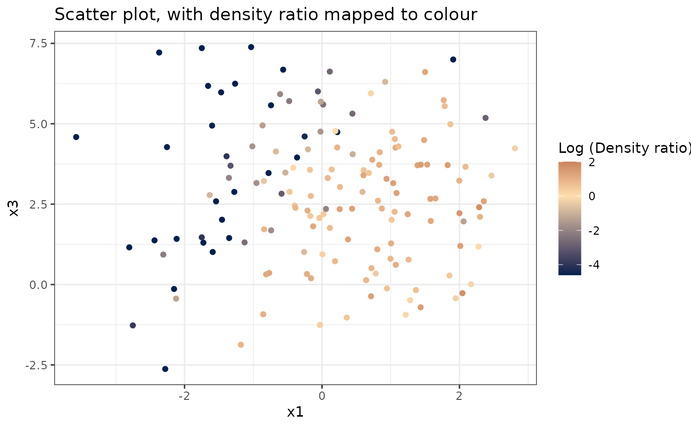
# Plot density ratio for each pair of variables
plot_bivariate(dr)
#> Warning: Negative estimated density ratios for 12 observation(s) converted to 0.01 before applying logarithmic transformation
#> [[1]]
 #>
#> [[2]]
#>
#> [[2]]
 #>
#> [[3]]
#>
#> [[3]]
 #>
# Predict density ratio and inspect first 6 predictions
head(predict(dr))
#> , , 1
#>
#> [,1]
#> [1,] 2.1625009
#> [2,] 3.6694722
#> [3,] 2.7969688
#> [4,] 4.1387638
#> [5,] 0.1585054
#> [6,] 1.2616673
#>
#>
# Predict density ratio and inspect first 6 predictions
head(predict(dr))
#> , , 1
#>
#> [,1]
#> [1,] 2.1625009
#> [2,] 3.6694722
#> [3,] 2.7969688
#> [4,] 4.1387638
#> [5,] 0.1585054
#> [6,] 1.2616673
#>