Print a summary.spectral object
Examples
set.seed(123)
# Fit model
dr <- spectral(numerator_small, denominator_small)
# Inspect model object
dr
#>
#> Call:
#> spectral(df_numerator = numerator_small, df_denominator = denominator_small)
#>
#> Kernel Information:
#> Kernel type: Gaussian with L2 norm distances
#> Number of kernels: 100
#> sigma: num [1:10] 0.807 1.191 1.455 1.688 1.913 ...
#>
#>
#> Subspace dimension (J): num [1:50] 1 2 4 6 8 10 11 13 15 17 ...
#>
#> Optimal sigma: 3.582214
#> Optimal subspace: 8
#> Optimal kernel weights (cv): num [1:8] 1.0045 -0.6689 -0.0938 0.8499 0.0228 ...
#>
# Obtain summary of model object
summary(dr)
#>
#> Call:
#> spectral(df_numerator = numerator_small, df_denominator = denominator_small)
#>
#> Kernel Information:
#> Kernel type: Gaussian with L2 norm distances
#> Number of kernels: 100
#>
#> Optimal sigma: 3.582214
#> Optimal subspace: 8
#> Optimal kernel weights (cv): num [1:8] 1.0045 -0.6689 -0.0938 0.8499 0.0228 ...
#>
#> Pearson divergence between P(nu) and P(de): 0.8063
#> For a two-sample homogeneity test, use 'summary(x, test = TRUE)'.
#>
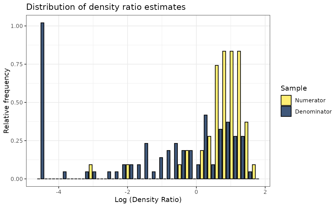
# Plot model object
plot(dr)
#> Warning: Negative estimated density ratios for 22 observation(s) converted to 0.01 before applying logarithmic transformation
#> `stat_bin()` using `bins = 30`. Pick better value `binwidth`.
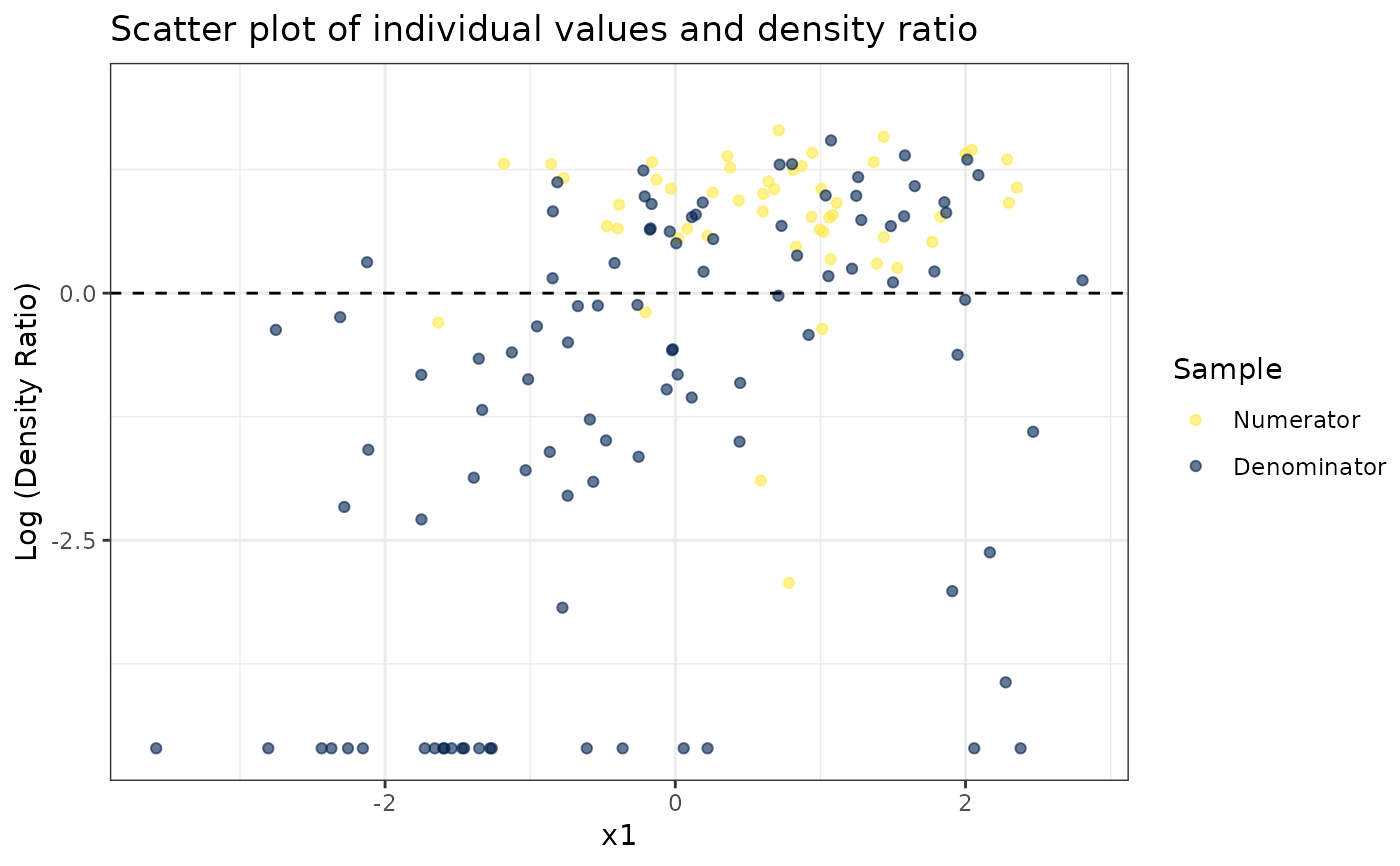
 # Plot density ratio for each variable individually
plot_univariate(dr)
#> Warning: Negative estimated density ratios for 22 observation(s) converted to 0.01 before applying logarithmic transformation
#> [[1]]
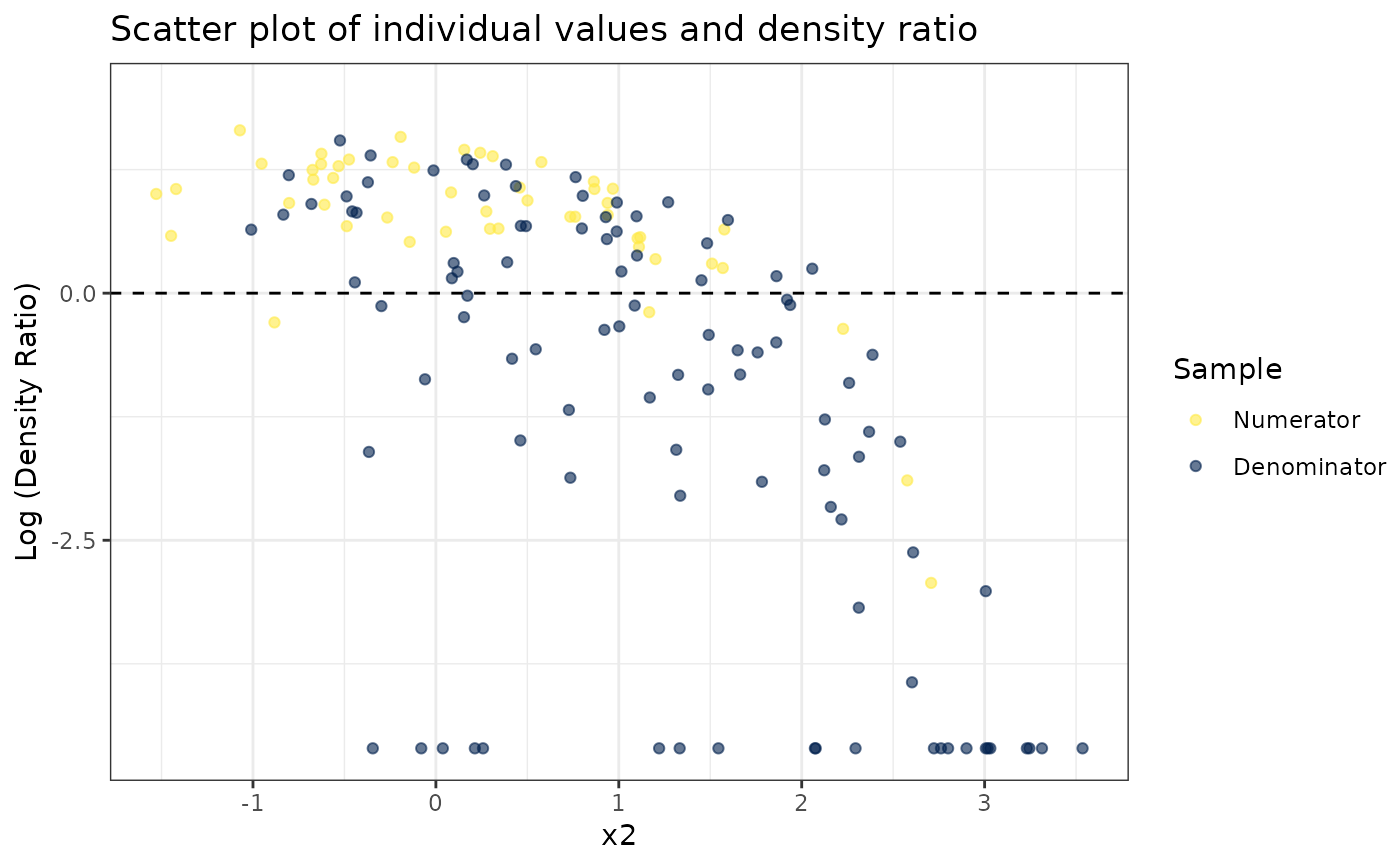
# Plot density ratio for each variable individually
plot_univariate(dr)
#> Warning: Negative estimated density ratios for 22 observation(s) converted to 0.01 before applying logarithmic transformation
#> [[1]]
 #>
#> [[2]]
#>
#> [[2]]
 #>
#> [[3]]
#>
#> [[3]]
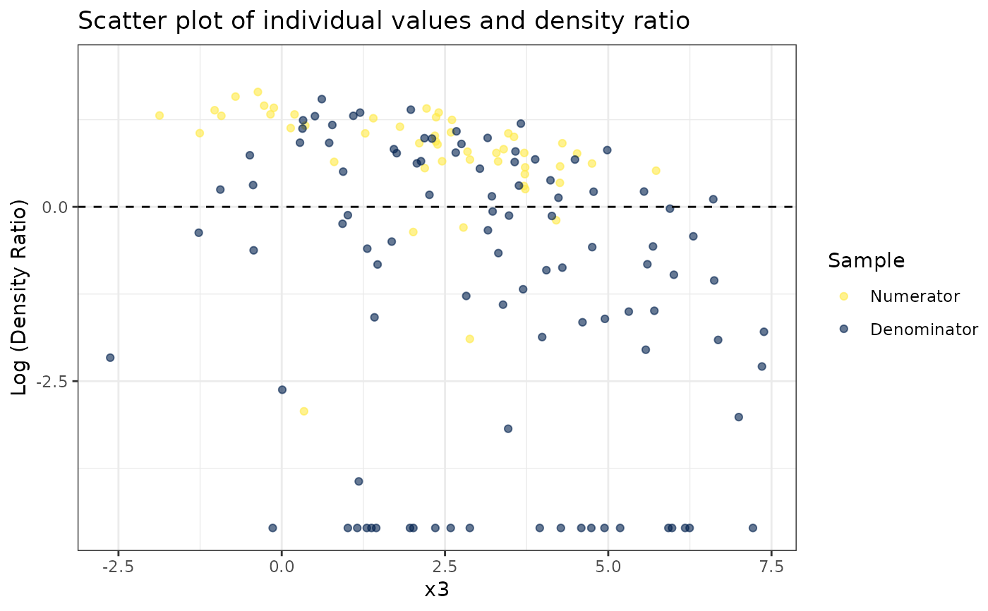 #>
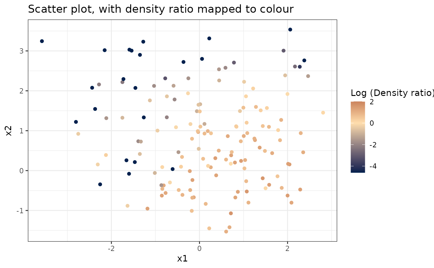
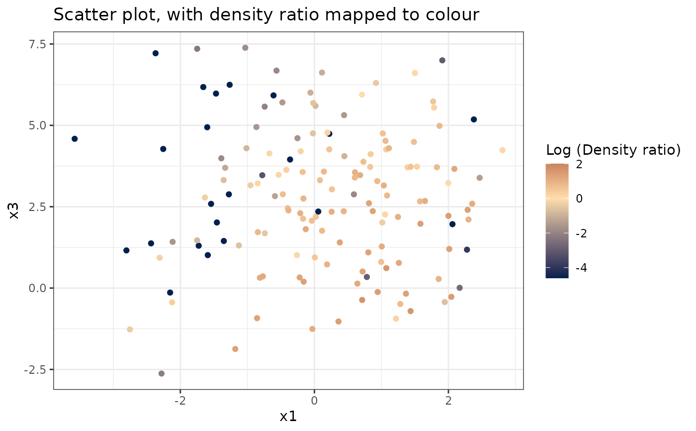
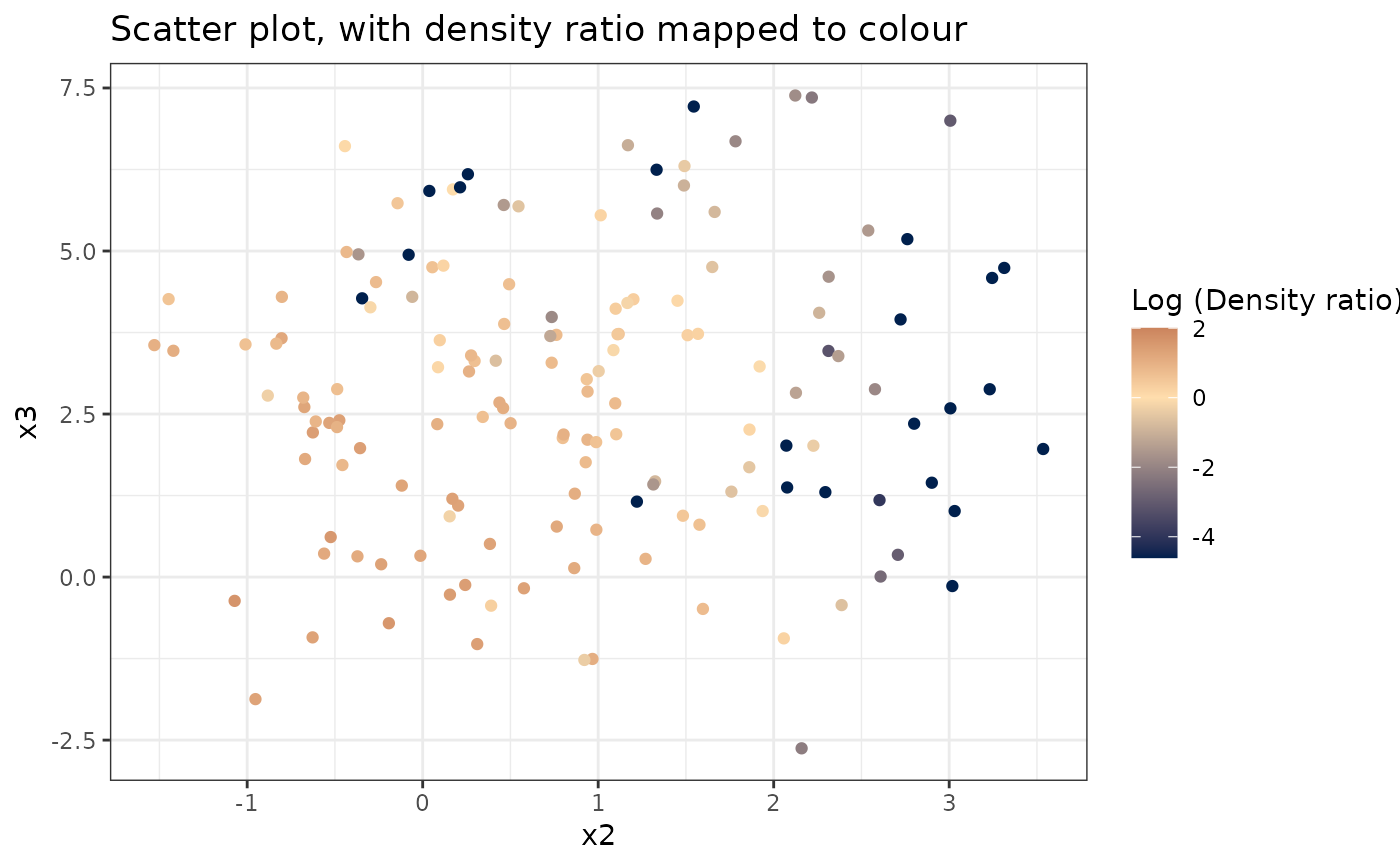
# Plot density ratio for each pair of variables
plot_bivariate(dr)
#> Warning: Negative estimated density ratios for 22 observation(s) converted to 0.01 before applying logarithmic transformation
#> [[1]]
#>
# Plot density ratio for each pair of variables
plot_bivariate(dr)
#> Warning: Negative estimated density ratios for 22 observation(s) converted to 0.01 before applying logarithmic transformation
#> [[1]]
 #>
#> [[2]]
#>
#> [[2]]
 #>
#> [[3]]
#>
#> [[3]]
 #>
# Predict density ratio and inspect first 6 predictions
head(predict(dr))
#> , , 1
#>
#> [,1]
#> [1,] 2.8779372
#> [2,] 3.8658889
#> [3,] 3.7674156
#> [4,] 4.8603842
#> [5,] 0.6970124
#> [6,] 2.1671079
#>
# Fit model with custom parameters
spectral(numerator_small, denominator_small, sigma = 2)
#>
#> Call:
#> spectral(df_numerator = numerator_small, df_denominator = denominator_small, sigma = 2)
#>
#> Kernel Information:
#> Kernel type: Gaussian with L2 norm distances
#> Number of kernels: 100
#> sigma: num 2
#>
#>
#> Subspace dimension (J): num [1:50] 1 2 4 6 8 10 11 13 15 17 ...
#>
#> Optimal sigma: 2
#> Optimal subspace: 4
#> Optimal kernel weights (cv): num [1:4] 0.98 -0.8324 -0.0561 0.6471
#>
#>
# Predict density ratio and inspect first 6 predictions
head(predict(dr))
#> , , 1
#>
#> [,1]
#> [1,] 2.8779372
#> [2,] 3.8658889
#> [3,] 3.7674156
#> [4,] 4.8603842
#> [5,] 0.6970124
#> [6,] 2.1671079
#>
# Fit model with custom parameters
spectral(numerator_small, denominator_small, sigma = 2)
#>
#> Call:
#> spectral(df_numerator = numerator_small, df_denominator = denominator_small, sigma = 2)
#>
#> Kernel Information:
#> Kernel type: Gaussian with L2 norm distances
#> Number of kernels: 100
#> sigma: num 2
#>
#>
#> Subspace dimension (J): num [1:50] 1 2 4 6 8 10 11 13 15 17 ...
#>
#> Optimal sigma: 2
#> Optimal subspace: 4
#> Optimal kernel weights (cv): num [1:4] 0.98 -0.8324 -0.0561 0.6471
#>