Spectral series based density ratio estimation
Usage
spectral(
  df_numerator,
  df_denominator,
  m = NULL,
  scale = "numerator",
  nsigma = 10,
  sigma_quantile = NULL,
  sigma = NULL,
  ncenters = NULL,
  cv = TRUE,
  nfold = 10,
  parallel = FALSE,
  nthreads = NULL,
  progressbar = TRUE
)
Arguments
- df_numerator
data.framewith exclusively numeric variables with the numerator samples- df_denominator
data.framewith exclusively numeric variables with the denominator samples (must have the same variables asdf_denominator)- m
Integer vector indicating the number of eigenvectors to use in the spectral series expansion. Defaults to 50 evenly spaced values between 1 and the number of denominator samples (or the largest number of samples that can be used as centers in the cross-validation scheme).
- scale
"numerator","denominator", orNULL, indicating whether to standardize each numeric variable according to the numerator means and standard deviations, the denominator means and standard deviations, or apply no standardization at all.- nsigma
Integer indicating the number of sigma values (bandwidth parameter of the Gaussian kernel gram matrix) to use in cross-validation.
- sigma_quantile
NULLor numeric vector with probabilities to calculate the quantiles of the distance matrix to obtain sigma values. IfNULL,nsigmavalues between0.05and0.95are used.- sigma
NULLor a scalar value to determine the bandwidth of the Gaussian kernel gram matrix. IfNULL,nsigmavalues between0.05and0.95are used.- ncenters
integer If smaller than the number of denominator observations, an approximation to the eigenvector expansion based on only ncenters samples is performed, instead of the full expansion. This can be useful for large datasets. Defaults to
NULL, such that all denominator samples are used.- cv
logical indicating whether to use cross-validation to determine the optimal sigma value and the optimal number of eigenvectors.
- nfold
Integer indicating the number of folds to use in the cross-validation scheme. If
cvisFALSE, this parameter is ignored.- parallel
logical indicating whether to use parallel processing in the cross-validation scheme.
- nthreads
NULLor integer indicating the number of threads to use for parallel processing. If parallel processing is enabled, it defaults to the number of available threads minus one.- progressbar
Logical indicating whether or not to display a progressbar.
Value
spectral-object, containing all information to calculate the
density ratio using optimal sigma and optimal spectral series expansion.
References
Izbicki, R., Lee, A. & Schafer, C. (2014). High-Dimensional Density Ratio Estimation with Extensions to Approximate Likelihood Computation. Proceedings of Machine Learning Research 33, 420-429. Available from https://proceedings.mlr.press/v33/izbicki14.html.
Examples
set.seed(123)
# Fit model
dr <- spectral(numerator_small, denominator_small)
# Inspect model object
dr
#>
#> Call:
#> spectral(df_numerator = numerator_small, df_denominator = denominator_small)
#>
#> Kernel Information:
#> Kernel type: Gaussian with L2 norm distances
#> Number of kernels: 100
#> sigma: num [1:10] 0.807 1.191 1.455 1.688 1.913 ...
#>
#>
#> Subspace dimension (J): num [1:50] 1 2 4 6 8 10 11 13 15 17 ...
#>
#> Optimal sigma: 3.582214
#> Optimal subspace: 8
#> Optimal kernel weights (cv): num [1:8] 1.0045 -0.6689 -0.0938 0.8499 0.0228 ...
#>
# Obtain summary of model object
summary(dr)
#>
#> Call:
#> spectral(df_numerator = numerator_small, df_denominator = denominator_small)
#>
#> Kernel Information:
#> Kernel type: Gaussian with L2 norm distances
#> Number of kernels: 100
#>
#> Optimal sigma: 3.582214
#> Optimal subspace: 8
#> Optimal kernel weights (cv): num [1:8] 1.0045 -0.6689 -0.0938 0.8499 0.0228 ...
#>
#> Pearson divergence between P(nu) and P(de): 0.8063
#> For a two-sample homogeneity test, use 'summary(x, test = TRUE)'.
#>
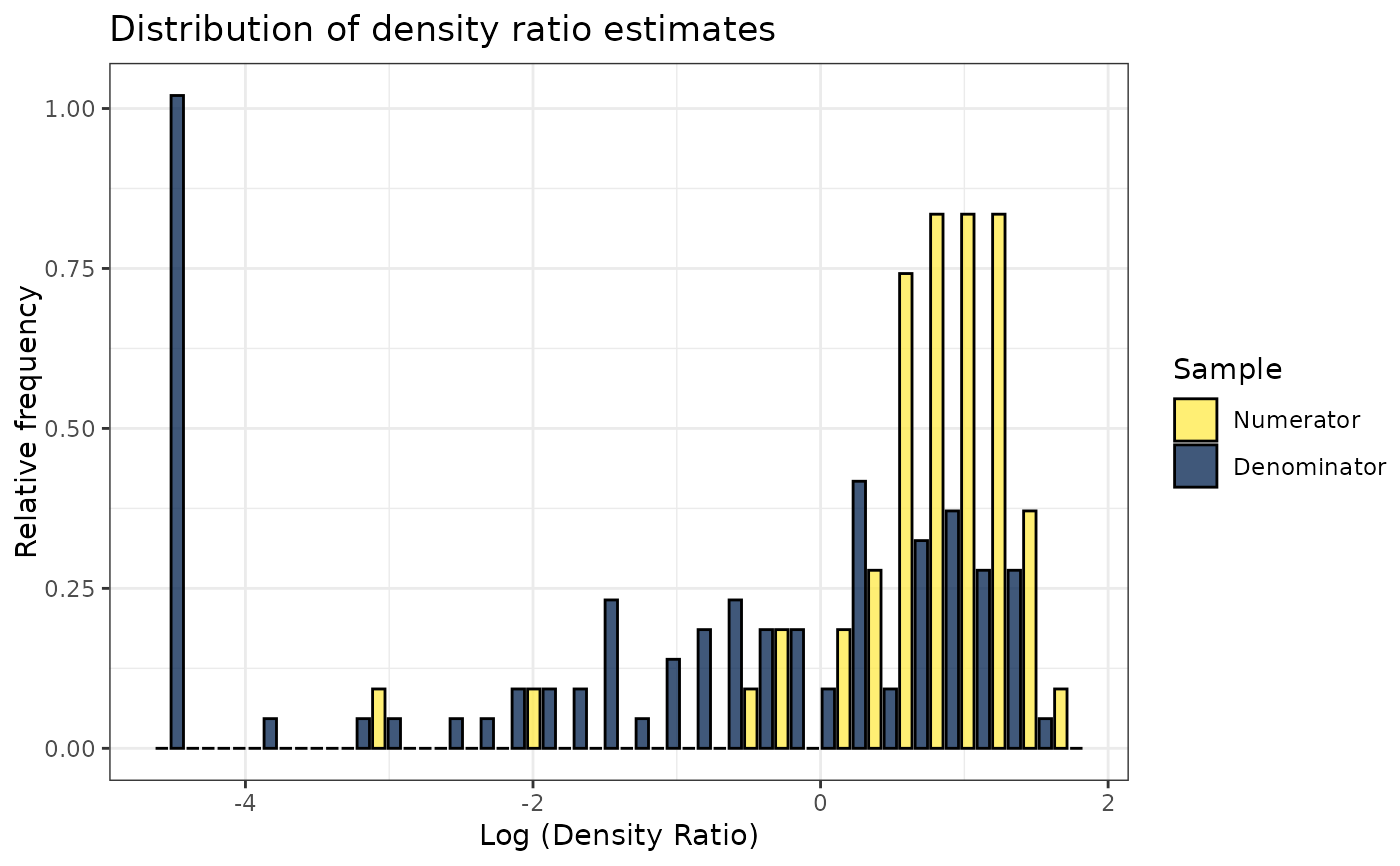
# Plot model object
plot(dr)
#> Warning: Negative estimated density ratios for 22 observation(s) converted to 0.01 before applying logarithmic transformation
#> `stat_bin()` using `bins = 30`. Pick better value `binwidth`.
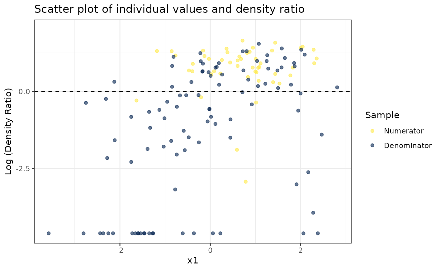
 # Plot density ratio for each variable individually
plot_univariate(dr)
#> Warning: Negative estimated density ratios for 22 observation(s) converted to 0.01 before applying logarithmic transformation
#> [[1]]
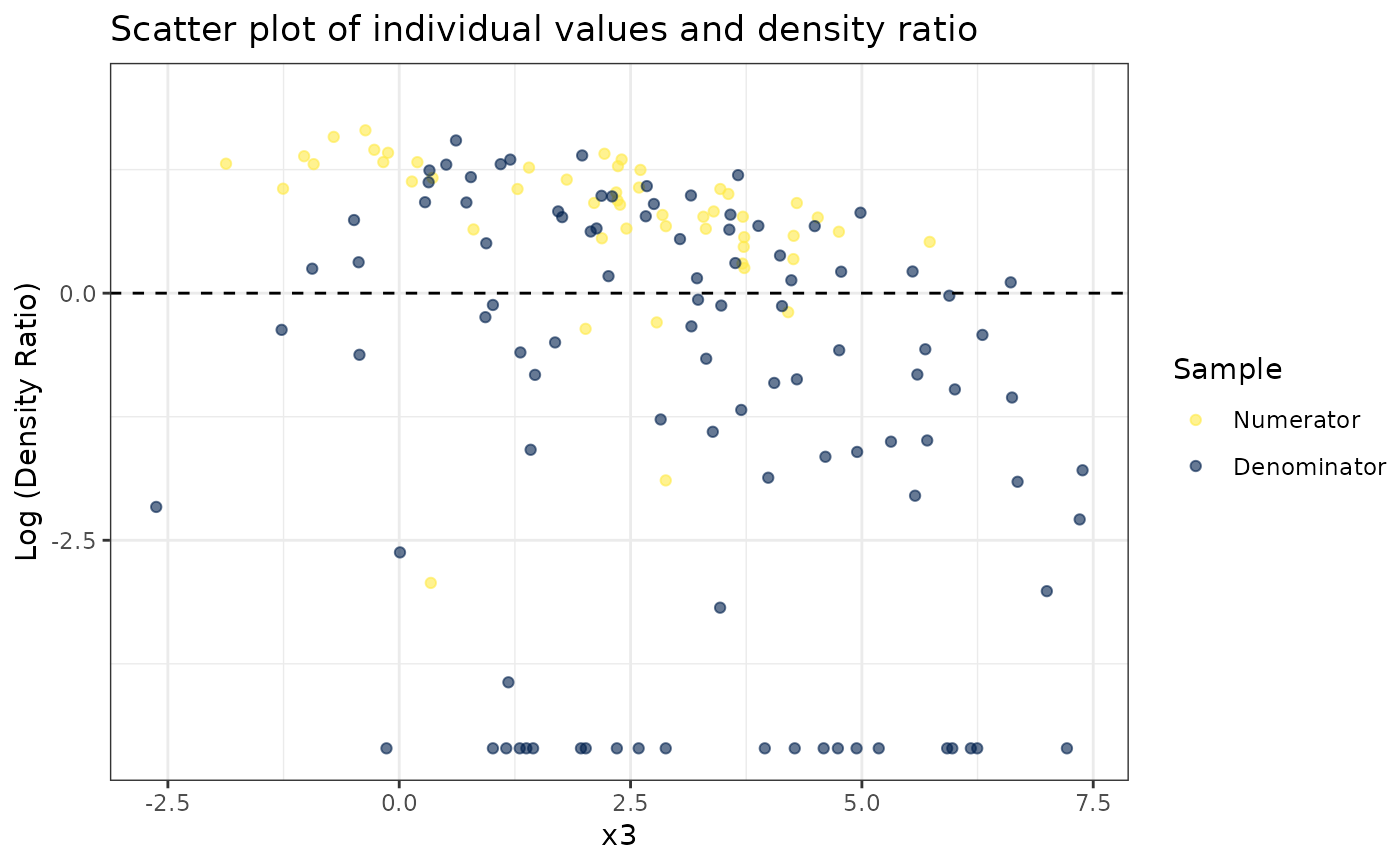
# Plot density ratio for each variable individually
plot_univariate(dr)
#> Warning: Negative estimated density ratios for 22 observation(s) converted to 0.01 before applying logarithmic transformation
#> [[1]]
 #>
#> [[2]]
#>
#> [[2]]
 #>
#> [[3]]
#>
#> [[3]]
 #>
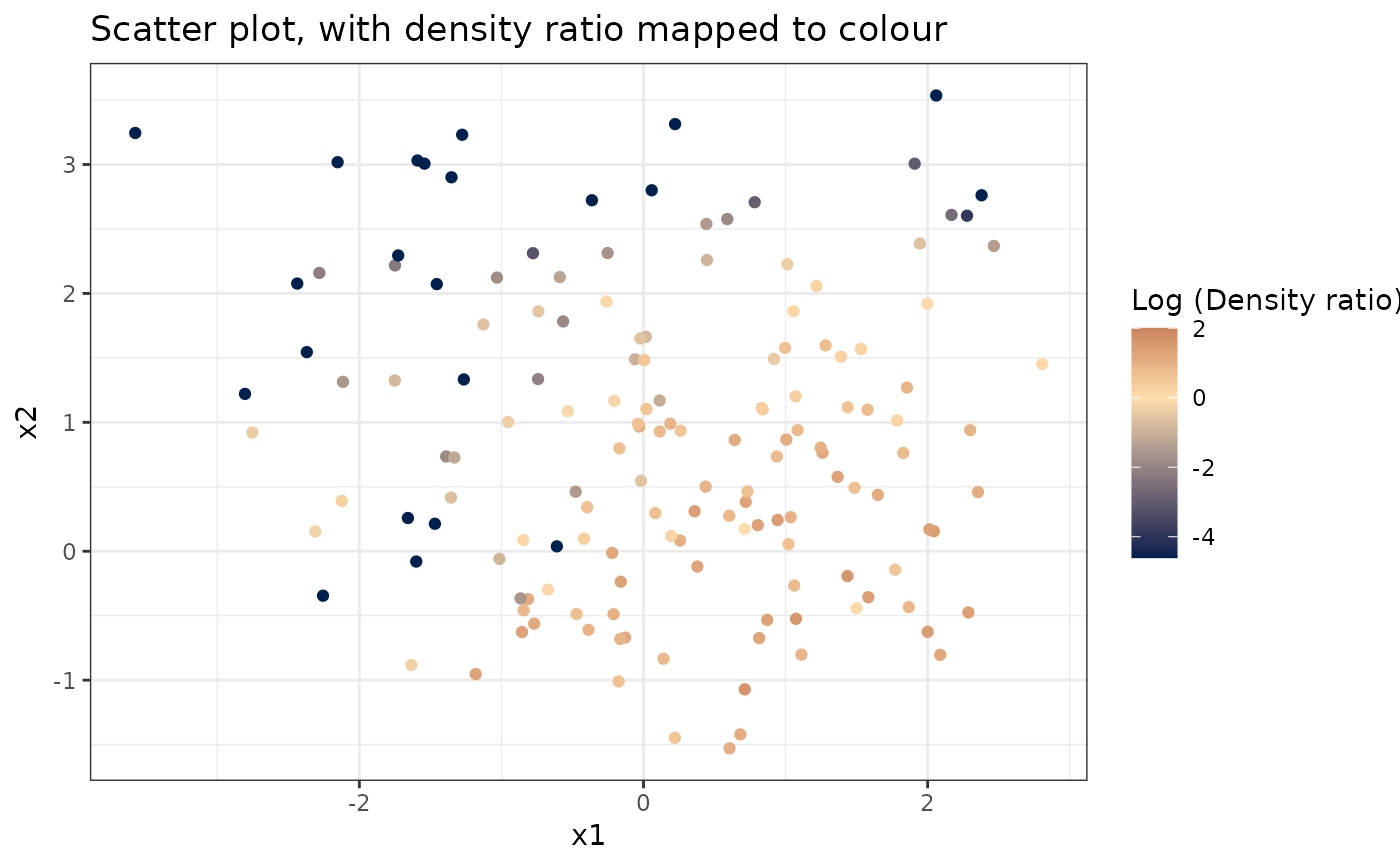
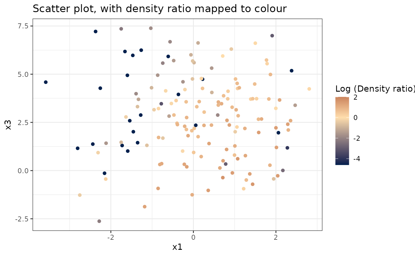
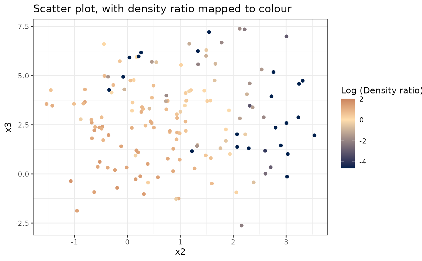
# Plot density ratio for each pair of variables
plot_bivariate(dr)
#> Warning: Negative estimated density ratios for 22 observation(s) converted to 0.01 before applying logarithmic transformation
#> [[1]]
#>
# Plot density ratio for each pair of variables
plot_bivariate(dr)
#> Warning: Negative estimated density ratios for 22 observation(s) converted to 0.01 before applying logarithmic transformation
#> [[1]]
 #>
#> [[2]]
#>
#> [[2]]
 #>
#> [[3]]
#>
#> [[3]]
 #>
# Predict density ratio and inspect first 6 predictions
head(predict(dr))
#> , , 1
#>
#> [,1]
#> [1,] 2.8779372
#> [2,] 3.8658889
#> [3,] 3.7674156
#> [4,] 4.8603842
#> [5,] 0.6970124
#> [6,] 2.1671079
#>
# Fit model with custom parameters
spectral(numerator_small, denominator_small, sigma = 2)
#>
#> Call:
#> spectral(df_numerator = numerator_small, df_denominator = denominator_small, sigma = 2)
#>
#> Kernel Information:
#> Kernel type: Gaussian with L2 norm distances
#> Number of kernels: 100
#> sigma: num 2
#>
#>
#> Subspace dimension (J): num [1:50] 1 2 4 6 8 10 11 13 15 17 ...
#>
#> Optimal sigma: 2
#> Optimal subspace: 4
#> Optimal kernel weights (cv): num [1:4] 0.98 -0.8324 -0.0561 0.6471
#>
#>
# Predict density ratio and inspect first 6 predictions
head(predict(dr))
#> , , 1
#>
#> [,1]
#> [1,] 2.8779372
#> [2,] 3.8658889
#> [3,] 3.7674156
#> [4,] 4.8603842
#> [5,] 0.6970124
#> [6,] 2.1671079
#>
# Fit model with custom parameters
spectral(numerator_small, denominator_small, sigma = 2)
#>
#> Call:
#> spectral(df_numerator = numerator_small, df_denominator = denominator_small, sigma = 2)
#>
#> Kernel Information:
#> Kernel type: Gaussian with L2 norm distances
#> Number of kernels: 100
#> sigma: num 2
#>
#>
#> Subspace dimension (J): num [1:50] 1 2 4 6 8 10 11 13 15 17 ...
#>
#> Optimal sigma: 2
#> Optimal subspace: 4
#> Optimal kernel weights (cv): num [1:4] 0.98 -0.8324 -0.0561 0.6471
#>