Print a kmm object
Examples
set.seed(123)
# Fit model
dr <- kmm(numerator_small, denominator_small)
# Inspect model object
dr
#>
#> Call:
#> kmm(df_numerator = numerator_small, df_denominator = denominator_small)
#>
#> Kernel Information:
#> Kernel type: Gaussian with L2 norm distances
#> Number of kernels: 150
#> sigma: num [1:10] 0.801 1.2 1.483 1.723 1.954 ...
#>
#> Optimal sigma (5-fold cv): 3.67
#> Optimal kernel weights (5-fold cv): num [1:150, 1] 0.23 0.416 -0.166 1.512 0.831 ...
#>
#> Optimization parameters:
#> Optimization method: Unconstrained
#>
# Obtain summary of model object
summary(dr)
#>
#> Call:
#> kmm(df_numerator = numerator_small, df_denominator = denominator_small)
#>
#> Kernel Information:
#> Kernel type: Gaussian with L2 norm distances
#> Number of kernels: 150
#> Optimal sigma: 3.669758
#> Optimal kernel weights: num [1:150, 1] 0.23 0.416 -0.166 1.512 0.831 ...
#>
#> Pearson divergence between P(nu) and P(de): 0.9439
#> For a two-sample homogeneity test, use 'summary(x, test = TRUE)'.
#>
# Plot model object
plot(dr)
#> Warning: Negative estimated density ratios for 19 observation(s) converted to 0.01 before applying logarithmic transformation
#> `stat_bin()` using `bins = 30`. Pick better value `binwidth`.
 # Plot density ratio for each variable individually
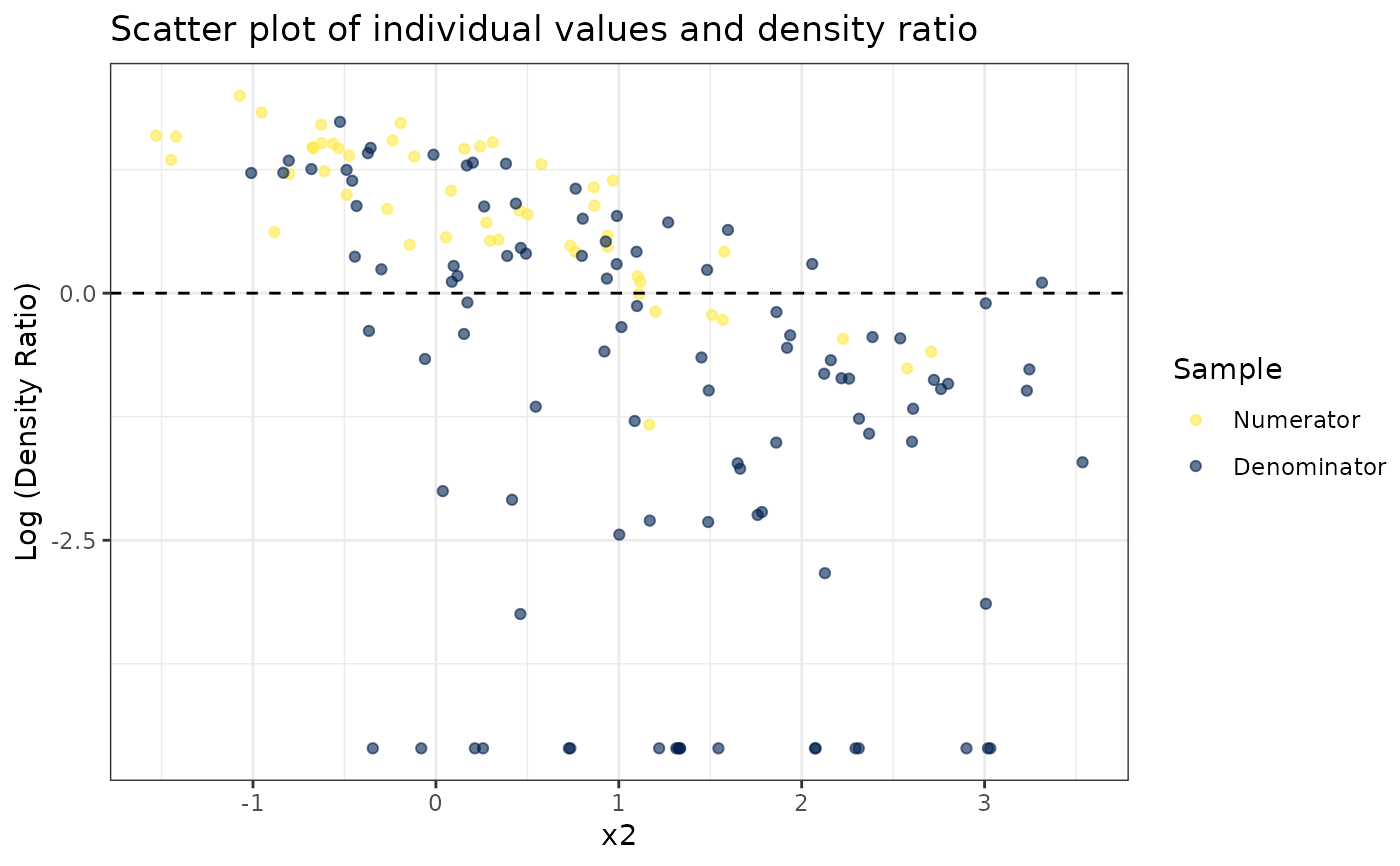
plot_univariate(dr)
#> Warning: Negative estimated density ratios for 19 observation(s) converted to 0.01 before applying logarithmic transformation
#> [[1]]
# Plot density ratio for each variable individually
plot_univariate(dr)
#> Warning: Negative estimated density ratios for 19 observation(s) converted to 0.01 before applying logarithmic transformation
#> [[1]]
 #>
#> [[2]]
#>
#> [[2]]
 #>
#> [[3]]
#>
#> [[3]]
 #>
# Plot density ratio for each pair of variables
plot_bivariate(dr)
#> Warning: Negative estimated density ratios for 19 observation(s) converted to 0.01 before applying logarithmic transformation
#> [[1]]
#>
# Plot density ratio for each pair of variables
plot_bivariate(dr)
#> Warning: Negative estimated density ratios for 19 observation(s) converted to 0.01 before applying logarithmic transformation
#> [[1]]
 #>
#> [[2]]
#>
#> [[2]]
 #>
#> [[3]]
#>
#> [[3]]
 #>
# Predict density ratio and inspect first 6 predictions
head(predict(dr))
#> [,1]
#> [1,] 3.1261579
#> [2,] 4.0233887
#> [3,] 3.6868339
#> [4,] 5.5934888
#> [5,] 0.6302996
#> [6,] 1.5225886
# Fit model with custom parameters
kmm(numerator_small, denominator_small,
nsigma = 4, ncenters = 50, nfold = 4,
constrained = TRUE)
#>
#> Call:
#> kmm(df_numerator = numerator_small, df_denominator = denominator_small, constrained = TRUE, nsigma = 4, ncenters = 50, nfold = 4)
#>
#> Kernel Information:
#> Kernel type: Gaussian with L2 norm distances
#> Number of kernels: 50
#> sigma: num [1:4] 0.822 1.795 2.475 3.711
#>
#> Optimal sigma (4-fold cv): 1.795
#> Optimal kernel weights (4-fold cv): num [1:50, 1] -0.000659 -0.000376 -0.001281 -0.000815 -0.001291 ...
#>
#> Optimization parameters:
#> Optimization method: Constrained
#>
#>
# Predict density ratio and inspect first 6 predictions
head(predict(dr))
#> [,1]
#> [1,] 3.1261579
#> [2,] 4.0233887
#> [3,] 3.6868339
#> [4,] 5.5934888
#> [5,] 0.6302996
#> [6,] 1.5225886
# Fit model with custom parameters
kmm(numerator_small, denominator_small,
nsigma = 4, ncenters = 50, nfold = 4,
constrained = TRUE)
#>
#> Call:
#> kmm(df_numerator = numerator_small, df_denominator = denominator_small, constrained = TRUE, nsigma = 4, ncenters = 50, nfold = 4)
#>
#> Kernel Information:
#> Kernel type: Gaussian with L2 norm distances
#> Number of kernels: 50
#> sigma: num [1:4] 0.822 1.795 2.475 3.711
#>
#> Optimal sigma (4-fold cv): 1.795
#> Optimal kernel weights (4-fold cv): num [1:50, 1] -0.000659 -0.000376 -0.001281 -0.000815 -0.001291 ...
#>
#> Optimization parameters:
#> Optimization method: Constrained
#>