Kernel mean matching approach to density ratio estimation
Usage
kmm(
  df_numerator,
  df_denominator,
  scale = "numerator",
  constrained = FALSE,
  nsigma = 10,
  sigma_quantile = NULL,
  sigma = NULL,
  ncenters = 200,
  centers = NULL,
  cv = TRUE,
  nfold = 5,
  parallel = FALSE,
  nthreads = NULL,
  progressbar = TRUE,
  osqp_settings = NULL,
  cluster = NULL
)
Arguments
- df_numerator
data.framewith exclusively numeric variables with the numerator samples- df_denominator
data.framewith exclusively numeric variables with the denominator samples (must have the same variables asdf_denominator)- scale
"numerator","denominator", orNULL, indicating whether to standardize each numeric variable according to the numerator means and standard deviations, the denominator means and standard deviations, or apply no standardization at all.- constrained
logicalequalsFALSEto use unconstrained optimization,TRUEto use constrained optimization. Defaults toFALSE.- nsigma
Integer indicating the number of sigma values (bandwidth parameter of the Gaussian kernel gram matrix) to use in cross-validation.
- sigma_quantile
NULLor numeric vector with probabilities to calculate the quantiles of the distance matrix to obtain sigma values. IfNULL,nsigmavalues between0.25and0.75are used.- sigma
NULLor a scalar value to determine the bandwidth of the Gaussian kernel gram matrix. IfNULL,nsigmavalues between0.25and0.75are used.- ncenters
integerMaximum number of Gaussian centers in the kernel gram matrix.- centers
NULLordata.framewith the same dimensions as the data, indicating the centers for the Gaussian kernel gram matrix.- cv
Logical indicating whether or not to do cross-validation
- nfold
Number of cross-validation folds used in order to calculate the optimal
sigmavalue (default is 5-fold cv).- parallel
logical indicating whether to use parallel processing in the cross-validation scheme.
- nthreads
NULLor integer indicating the number of threads to use for parallel processing. If parallel processing is enabled, it defaults to the number of available threads minus one.- progressbar
Logical indicating whether or not to display a progressbar.
- osqp_settings
Optional: settings to pass to the
osqpsolver for constrained optimization.- cluster
Optional: a cluster object to use for parallel processing, see
parallel::makeCluster.
Value
kmm-object, containing all information to calculate the
density ratio using optimal sigma and optimal weights.
References
Huang, J., Smola, A. J., Gretton, A., Borgwardt, K. M., & Schölkopf, B. (2006). Correcting sample selection bias by unlabeled data. In Advances in Neural Information Processing Systems, edited by B. Schölkopf, J. Platt and T. Hoffman. Available from https://proceedings.neurips.cc/paper/2006/hash/a2186aa7c086b46ad4e8bf81e2a3a19b-Abstract.html.
Examples
set.seed(123)
# Fit model
dr <- kmm(numerator_small, denominator_small)
# Inspect model object
dr
#>
#> Call:
#> kmm(df_numerator = numerator_small, df_denominator = denominator_small)
#>
#> Kernel Information:
#> Kernel type: Gaussian with L2 norm distances
#> Number of kernels: 150
#> sigma: num [1:10] 0.801 1.2 1.483 1.723 1.954 ...
#>
#> Optimal sigma (5-fold cv): 3.67
#> Optimal kernel weights (5-fold cv): num [1:150, 1] 0.23 0.416 -0.166 1.512 0.831 ...
#>
#> Optimization parameters:
#> Optimization method: Unconstrained
#>
# Obtain summary of model object
summary(dr)
#>
#> Call:
#> kmm(df_numerator = numerator_small, df_denominator = denominator_small)
#>
#> Kernel Information:
#> Kernel type: Gaussian with L2 norm distances
#> Number of kernels: 150
#> Optimal sigma: 3.669758
#> Optimal kernel weights: num [1:150, 1] 0.23 0.416 -0.166 1.512 0.831 ...
#>
#> Pearson divergence between P(nu) and P(de): 0.9439
#> For a two-sample homogeneity test, use 'summary(x, test = TRUE)'.
#>
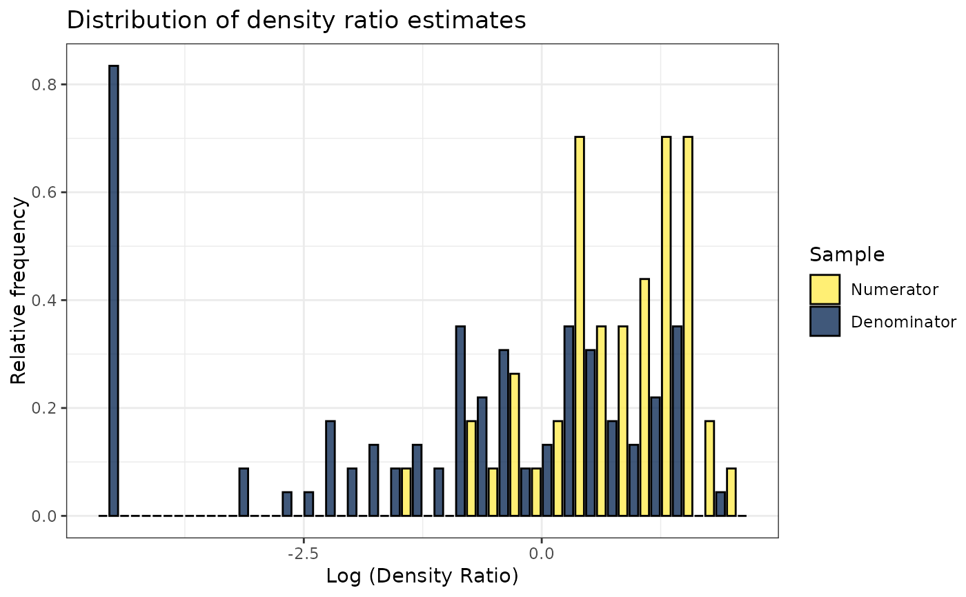
# Plot model object
plot(dr)
#> Warning: Negative estimated density ratios for 19 observation(s) converted to 0.01 before applying logarithmic transformation
#> `stat_bin()` using `bins = 30`. Pick better value `binwidth`.
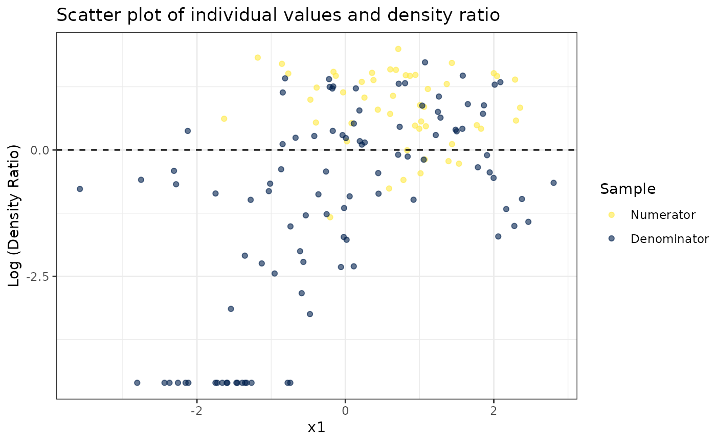
 # Plot density ratio for each variable individually
plot_univariate(dr)
#> Warning: Negative estimated density ratios for 19 observation(s) converted to 0.01 before applying logarithmic transformation
#> [[1]]
# Plot density ratio for each variable individually
plot_univariate(dr)
#> Warning: Negative estimated density ratios for 19 observation(s) converted to 0.01 before applying logarithmic transformation
#> [[1]]
 #>
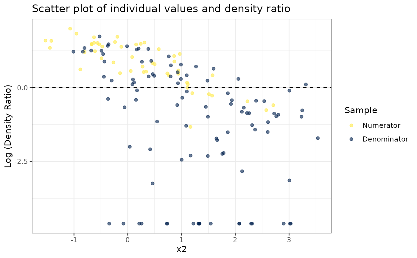
#> [[2]]
#>
#> [[2]]
 #>
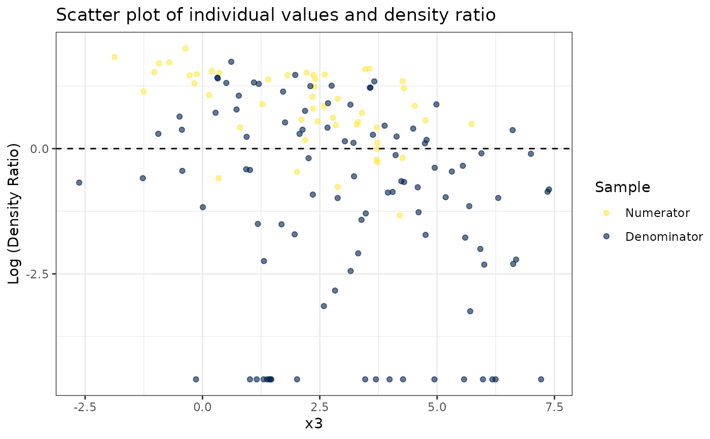
#> [[3]]
#>
#> [[3]]
 #>
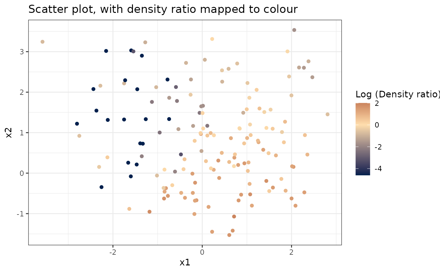
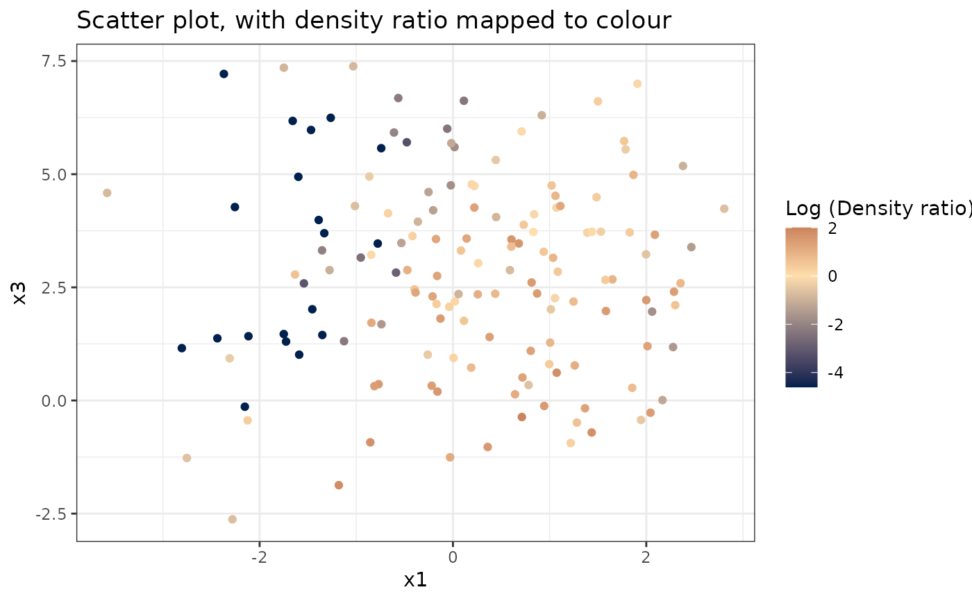
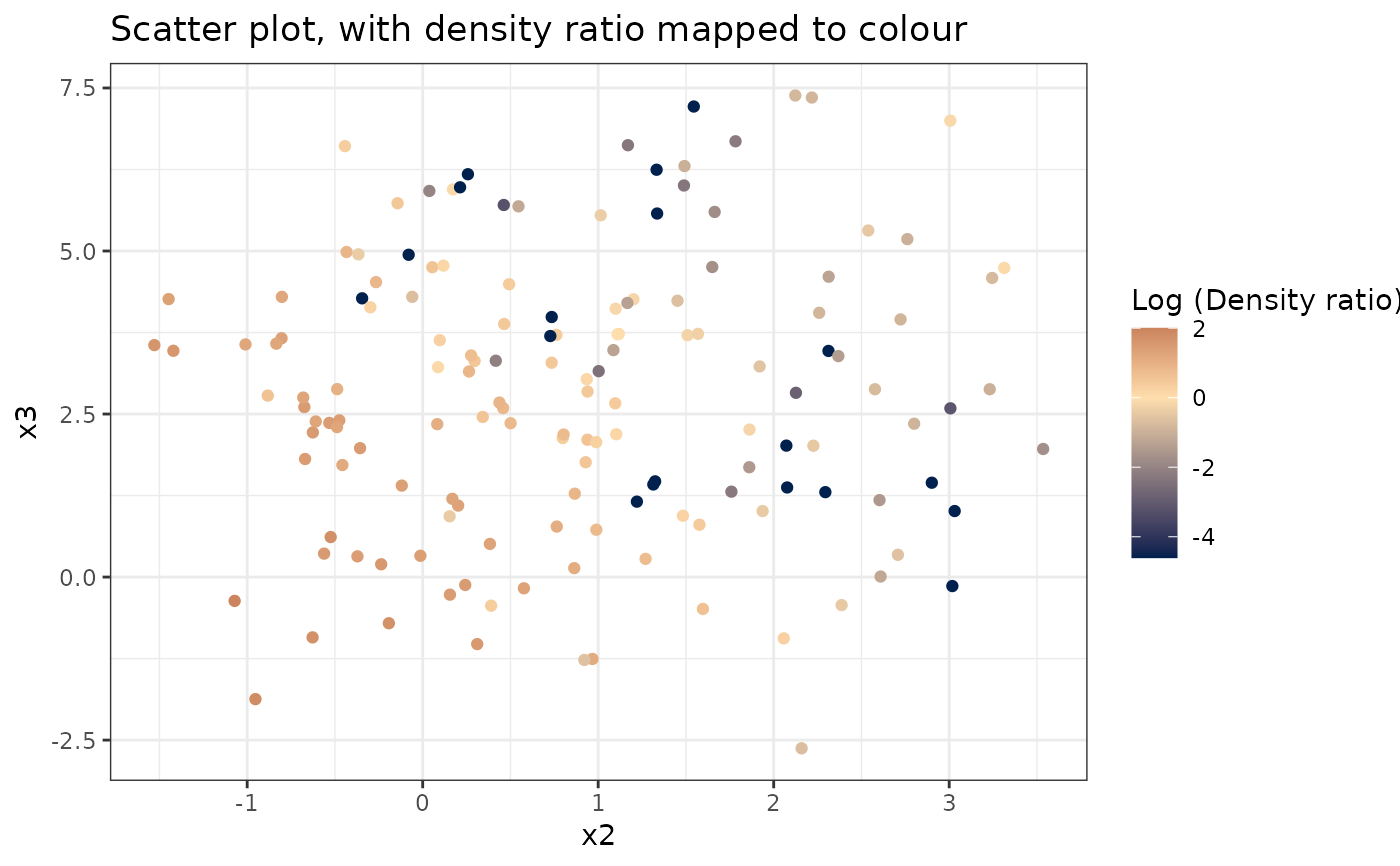
# Plot density ratio for each pair of variables
plot_bivariate(dr)
#> Warning: Negative estimated density ratios for 19 observation(s) converted to 0.01 before applying logarithmic transformation
#> [[1]]
#>
# Plot density ratio for each pair of variables
plot_bivariate(dr)
#> Warning: Negative estimated density ratios for 19 observation(s) converted to 0.01 before applying logarithmic transformation
#> [[1]]
 #>
#> [[2]]
#>
#> [[2]]
 #>
#> [[3]]
#>
#> [[3]]
 #>
# Predict density ratio and inspect first 6 predictions
head(predict(dr))
#> [,1]
#> [1,] 3.1261579
#> [2,] 4.0233887
#> [3,] 3.6868339
#> [4,] 5.5934888
#> [5,] 0.6302996
#> [6,] 1.5225886
# Fit model with custom parameters
kmm(numerator_small, denominator_small,
nsigma = 4, ncenters = 50, nfold = 4,
constrained = TRUE)
#>
#> Call:
#> kmm(df_numerator = numerator_small, df_denominator = denominator_small, constrained = TRUE, nsigma = 4, ncenters = 50, nfold = 4)
#>
#> Kernel Information:
#> Kernel type: Gaussian with L2 norm distances
#> Number of kernels: 50
#> sigma: num [1:4] 0.822 1.795 2.475 3.711
#>
#> Optimal sigma (4-fold cv): 1.795
#> Optimal kernel weights (4-fold cv): num [1:50, 1] -0.000659 -0.000376 -0.001281 -0.000815 -0.001291 ...
#>
#> Optimization parameters:
#> Optimization method: Constrained
#>
#>
# Predict density ratio and inspect first 6 predictions
head(predict(dr))
#> [,1]
#> [1,] 3.1261579
#> [2,] 4.0233887
#> [3,] 3.6868339
#> [4,] 5.5934888
#> [5,] 0.6302996
#> [6,] 1.5225886
# Fit model with custom parameters
kmm(numerator_small, denominator_small,
nsigma = 4, ncenters = 50, nfold = 4,
constrained = TRUE)
#>
#> Call:
#> kmm(df_numerator = numerator_small, df_denominator = denominator_small, constrained = TRUE, nsigma = 4, ncenters = 50, nfold = 4)
#>
#> Kernel Information:
#> Kernel type: Gaussian with L2 norm distances
#> Number of kernels: 50
#> sigma: num [1:4] 0.822 1.795 2.475 3.711
#>
#> Optimal sigma (4-fold cv): 1.795
#> Optimal kernel weights (4-fold cv): num [1:50, 1] -0.000659 -0.000376 -0.001281 -0.000815 -0.001291 ...
#>
#> Optimization parameters:
#> Optimization method: Constrained
#>