Obtain predicted density ratio values from a ulsif object

Obtain predicted density ratio values from a ulsif object

Usage

# S3 method for class 'ulsif'
predict(
  object,
  newdata = NULL,
  sigma = c("sigmaopt", "all"),
  lambda = c("lambdaopt", "all"),
  ...
)

Arguments

object

A ulsif object

newdata

Optional matrix new data set to compute the density

sigma

A scalar with the Gaussian kernel width

lambda

A scalar with the regularization parameter

...

Additional arguments to be passed to the function

Value

An array with predicted density ratio values from possibly new data, but otherwise the numerator samples.

See also

predict, ulsif

Examples

set.seed(123)
# Fit model
dr <- ulsif(numerator_small, denominator_small)
# Inspect model object
dr
#> 
#> Call:
#> ulsif(df_numerator = numerator_small, df_denominator = denominator_small)
#> 
#> Kernel Information:
#>   Kernel type: Gaussian with L2 norm distances
#>   Number of kernels: 150
#>   sigma: num [1:10] 0.711 1.08 1.333 1.538 1.742 ...
#> 
#> Regularization parameter (lambda): num [1:20] 1000 483.3 233.6 112.9 54.6 ...
#> 
#> Optimal sigma (loocv): 1.538158
#> Optimal lambda (loocv): 2.976351
#> Optimal kernel weights (loocv): num [1:151] 0.0666 0.0289 0.0423 0.0442 0.0454 ...
#>  
# Obtain summary of model object
summary(dr)
#> 
#> Call:
#> ulsif(df_numerator = numerator_small, df_denominator = denominator_small)
#> 
#> Kernel Information:
#>   Kernel type: Gaussian with L2 norm distances
#>   Number of kernels: 150
#> 
#> Optimal sigma: 1.538158
#> Optimal lambda: 2.976351
#> Optimal kernel weights: num [1:151] 0.0666 0.0289 0.0423 0.0442 0.0454 ...
#>  
#> Pearson divergence between P(nu) and P(de): 0.3868
#> For a two-sample homogeneity test, use 'summary(x, test = TRUE)'.
#> 
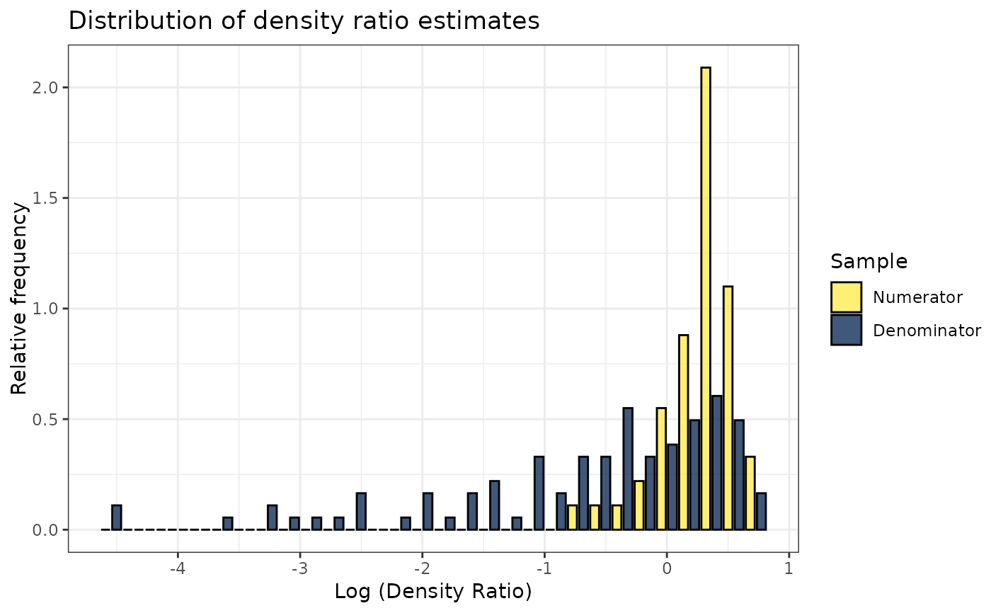
# Plot model object
plot(dr)
#> Warning: Negative estimated density ratios for 2 observation(s) converted to 0.01 before applying logarithmic transformation
#> `stat_bin()` using `bins = 30`. Pick better value with `binwidth`.

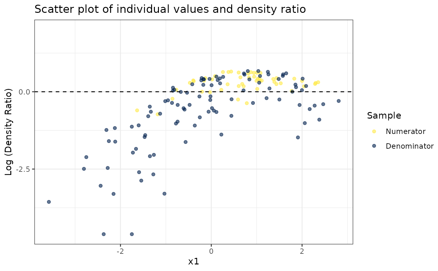
# Plot density ratio for each variable individually
plot_univariate(dr)
#> Warning: Negative estimated density ratios for 2 observation(s) converted to 0.01 before applying logarithmic transformation
#> [[1]]

#> 
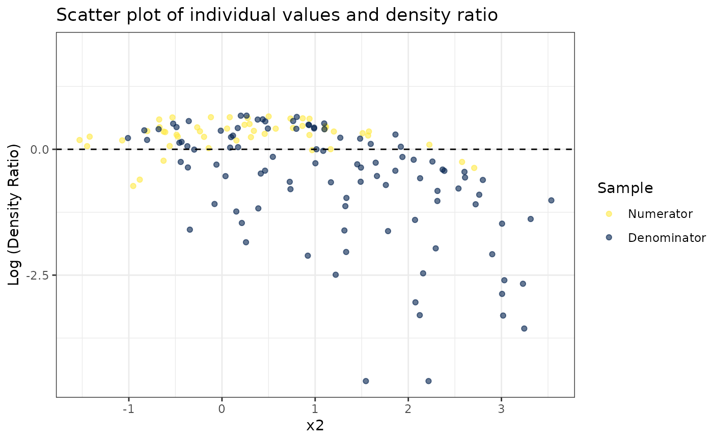
#> [[2]]

#> 
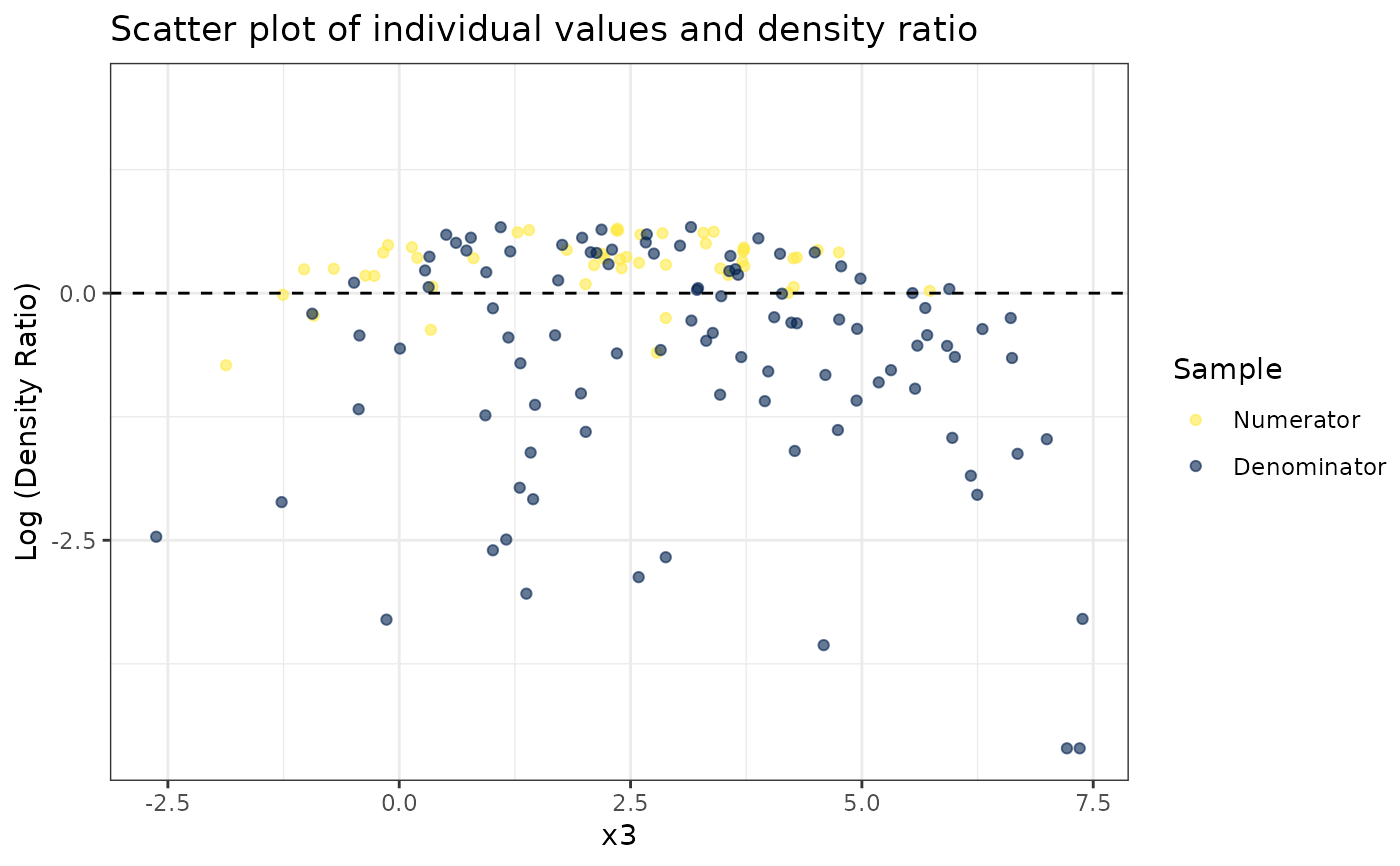
#> [[3]]

#> 
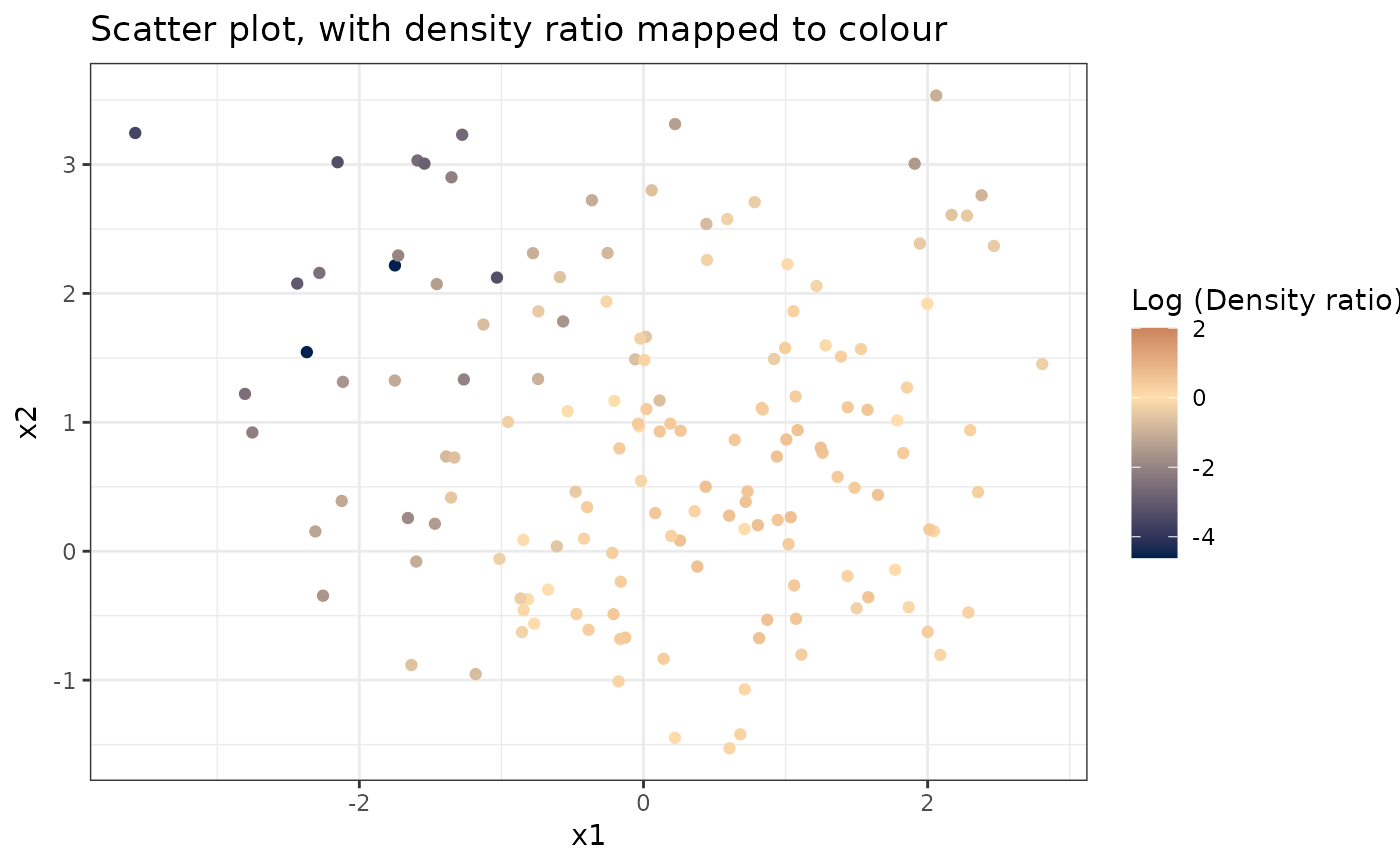
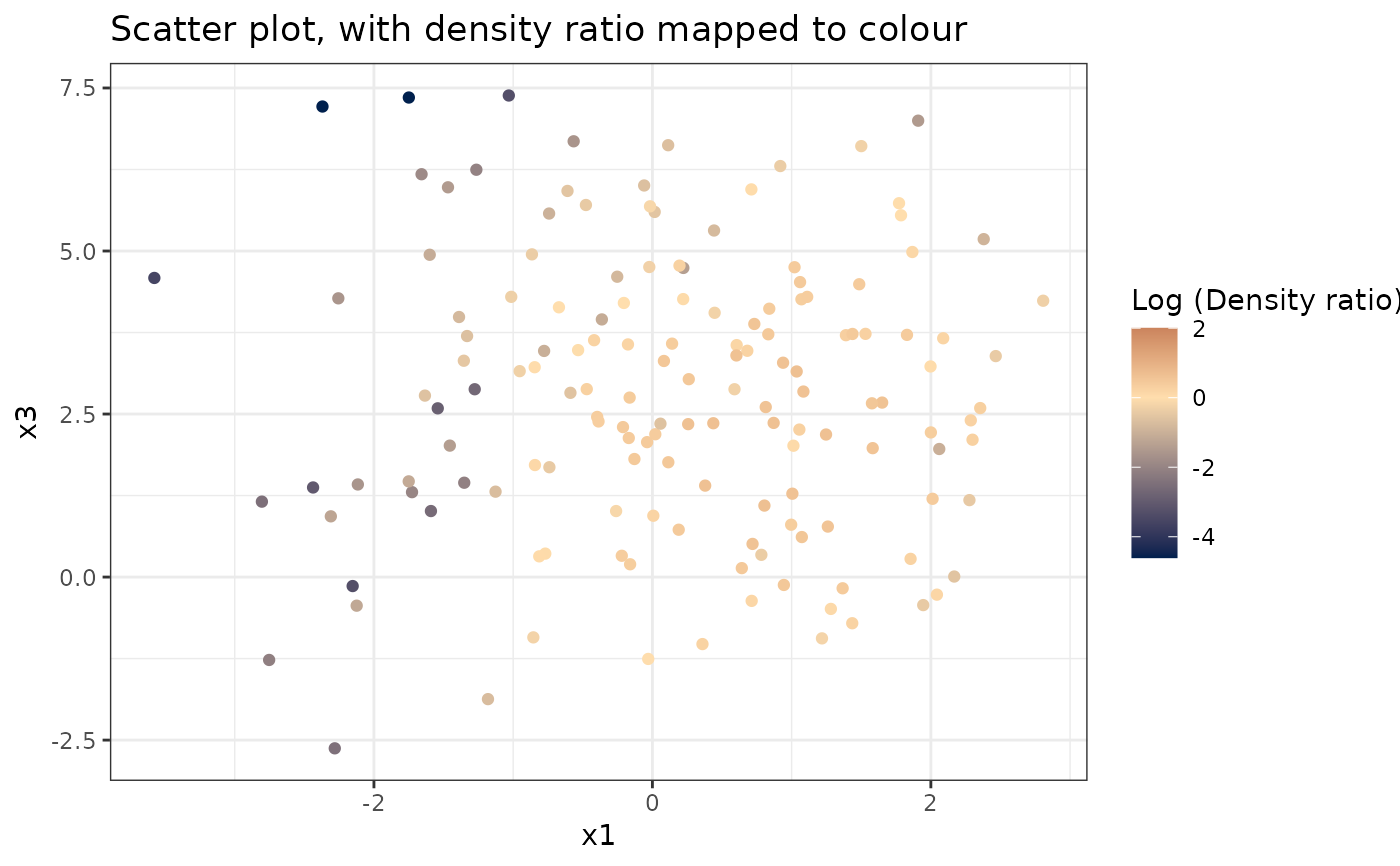
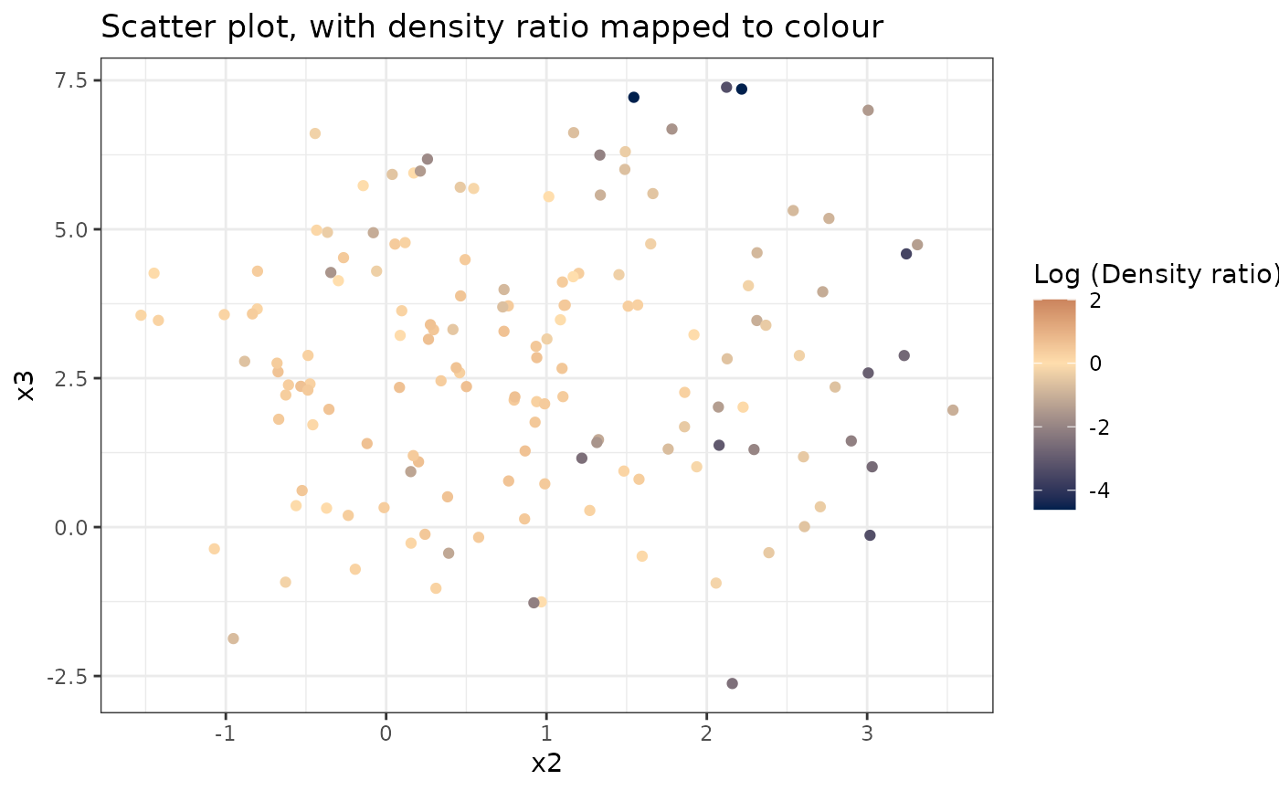
# Plot density ratio for each pair of variables
plot_bivariate(dr)
#> Warning: Negative estimated density ratios for 2 observation(s) converted to 0.01 before applying logarithmic transformation
#> [[1]]

#> 
#> [[2]]

#> 
#> [[3]]

#> 
# Predict density ratio and inspect first 6 predictions
head(predict(dr))
#> , , 1
#> 
#>           [,1]
#> [1,] 0.9838195
#> [2,] 1.2872509
#> [3,] 1.5069634
#> [4,] 1.2804095
#> [5,] 1.0953012
#> [6,] 1.5262485
#> 
# Fit model with custom parameters
ulsif(numerator_small, denominator_small, sigma = 2, lambda = 2)
#> 
#> Call:
#> ulsif(df_numerator = numerator_small, df_denominator = denominator_small,     sigma = 2, lambda = 2)
#> 
#> Kernel Information:
#>   Kernel type: Gaussian with L2 norm distances
#>   Number of kernels: 150
#>   sigma: num 2
#> 
#> Regularization parameter (lambda): num 2
#> 
#> Optimal sigma (loocv): 2
#> Optimal lambda (loocv): 2
#> Optimal kernel weights (loocv): num [1:151] 0.0378 0.0348 0.0554 0.053 0.0619 ...
#>