Unconstrained least-squares importance fitting
Usage
ulsif(
  df_numerator,
  df_denominator,
  intercept = FALSE,
  scale = "numerator",
  nsigma = 10,
  sigma_quantile = NULL,
  sigma = NULL,
  nlambda = 20,
  lambda = NULL,
  ncenters = 200,
  centers = NULL,
  parallel = FALSE,
  nthreads = NULL,
  progressbar = TRUE
)
Arguments
- df_numerator
data.framewith exclusively numeric variables with the numerator samples- df_denominator
data.framewith exclusively numeric variables with the denominator samples (must have the same variables asdf_denominator)- intercept
logicalIndicating whether to include an intercept term in the model. Defaults toFALSE.- scale
"numerator","denominator", orNULL, indicating whether to standardize each numeric variable according to the numerator means and standard deviations, the denominator means and standard deviations, or apply no standardization at all.- nsigma
Integer indicating the number of sigma values (bandwidth parameter of the Gaussian kernel gram matrix) to use in cross-validation.
- sigma_quantile
NULLor numeric vector with probabilities to calculate the quantiles of the distance matrix to obtain sigma values. IfNULL,nsigmavalues between0.05and0.95are used.- sigma
NULLor a scalar value to determine the bandwidth of the Gaussian kernel gram matrix. IfNULL,nsigmavalues between0.05and0.95are used.- nlambda
Integer indicating the number of
lambdavalues (regularization parameter), by default,lambdais set to10^seq(3, -3, length.out = nlambda).- lambda
NULLor numeric vector indicating the lambda values to use in cross-validation- ncenters
integerMaximum number of Gaussian centers in the kernel gram matrix.- centers
NULLordata.framewith the same dimensions as the data, indicating the centers for the Gaussian kernel gram matrix.- parallel
logical indicating whether to use parallel processing in the cross-validation scheme.
- nthreads
NULLor integer indicating the number of threads to use for parallel processing. If parallel processing is enabled, it defaults to the number of available threads minus one.- progressbar
Logical indicating whether or not to display a progressbar.
Value
ulsif-object, containing all information to calculate the
density ratio using optimal sigma and optimal weights.
References
Kanamori, T., Hido, S., & Sugiyama, M. (2009). A least-squares approach to direct importance estimation. Journal of Machine Learning Research, 10, 1391-1445. Available from https://jmlr.org/papers/v10/kanamori09a.html
Examples
set.seed(123)
# Fit model
dr <- ulsif(numerator_small, denominator_small)
# Inspect model object
dr
#>
#> Call:
#> ulsif(df_numerator = numerator_small, df_denominator = denominator_small)
#>
#> Kernel Information:
#> Kernel type: Gaussian with L2 norm distances
#> Number of kernels: 150
#> sigma: num [1:10] 0.711 1.08 1.333 1.538 1.742 ...
#>
#> Regularization parameter (lambda): num [1:20] 1000 483.3 233.6 112.9 54.6 ...
#>
#> Optimal sigma (loocv): 3.425852
#> Optimal lambda (loocv): 0.6951928
#> Optimal kernel weights (loocv): num [1:150] 0.05072 0.09115 0.07853 0.10771 -0.00969 ...
#>
# Obtain summary of model object
summary(dr)
#>
#> Call:
#> ulsif(df_numerator = numerator_small, df_denominator = denominator_small)
#>
#> Kernel Information:
#> Kernel type: Gaussian with L2 norm distances
#> Number of kernels: 150
#>
#> Optimal sigma: 3.425852
#> Optimal lambda: 0.6951928
#> Optimal kernel weights: num [1:150] 0.05072 0.09115 0.07853 0.10771 -0.00969 ...
#>
#> Pearson divergence between P(nu) and P(de): 0.3872
#> For a two-sample homogeneity test, use 'summary(x, test = TRUE)'.
#>
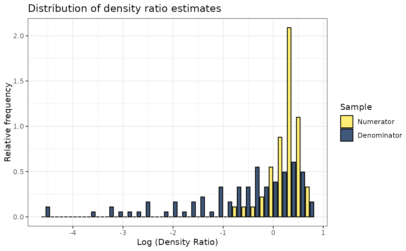
# Plot model object
plot(dr)
#> Warning: Negative estimated density ratios for 7 observation(s) converted to 0.01 before applying logarithmic transformation
#> `stat_bin()` using `bins = 30`. Pick better value `binwidth`.
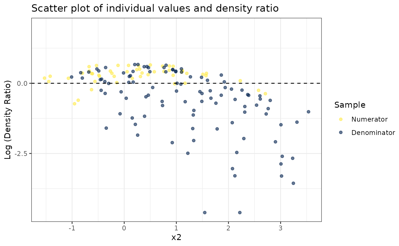
 # Plot density ratio for each variable individually
plot_univariate(dr)
#> Warning: Negative estimated density ratios for 7 observation(s) converted to 0.01 before applying logarithmic transformation
#> [[1]]
# Plot density ratio for each variable individually
plot_univariate(dr)
#> Warning: Negative estimated density ratios for 7 observation(s) converted to 0.01 before applying logarithmic transformation
#> [[1]]
 #>
#> [[2]]
#>
#> [[2]]
 #>
#> [[3]]
#>
#> [[3]]
 #>
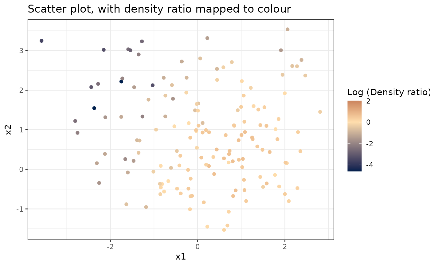
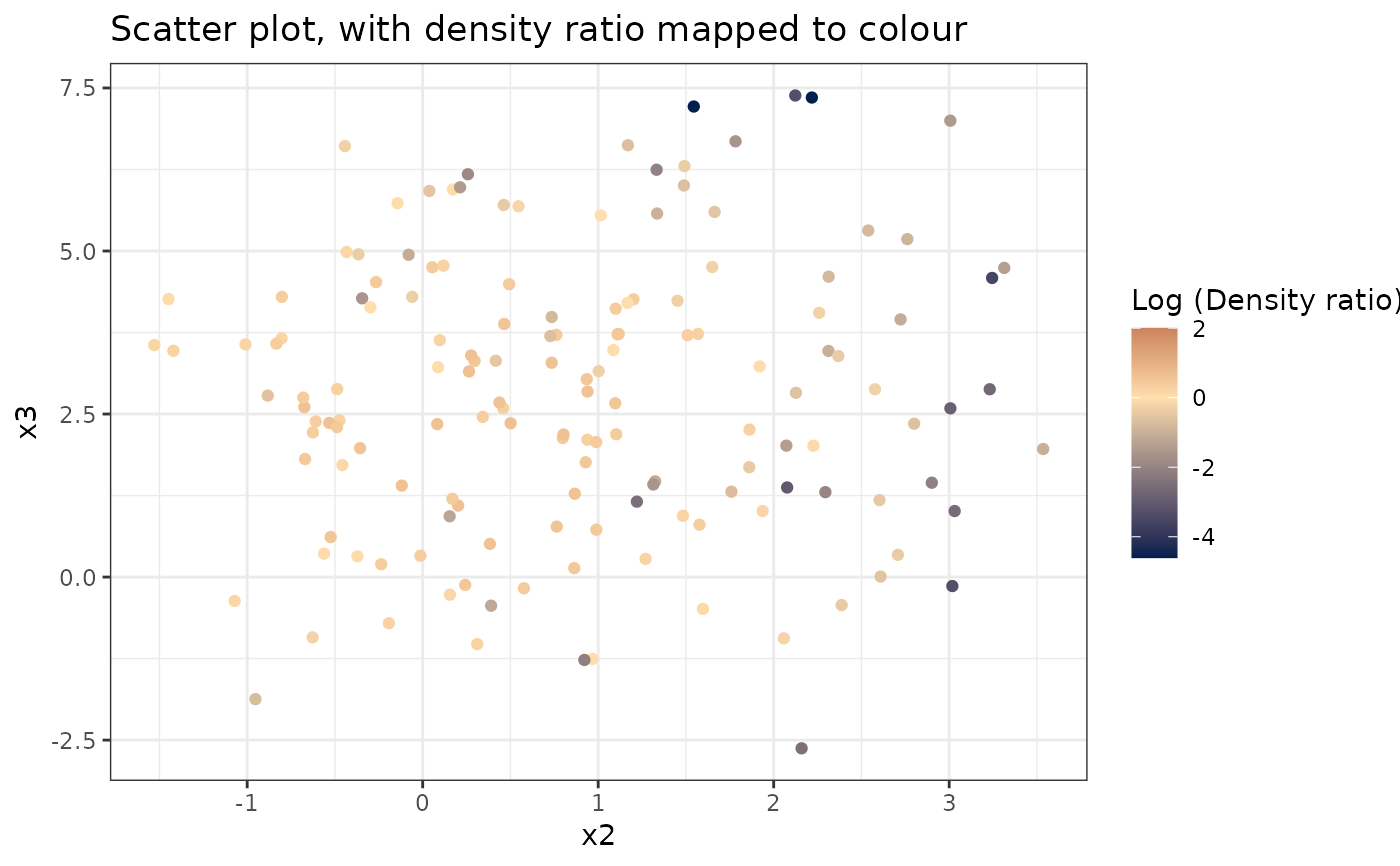
# Plot density ratio for each pair of variables
plot_bivariate(dr)
#> Warning: Negative estimated density ratios for 7 observation(s) converted to 0.01 before applying logarithmic transformation
#> [[1]]
#>
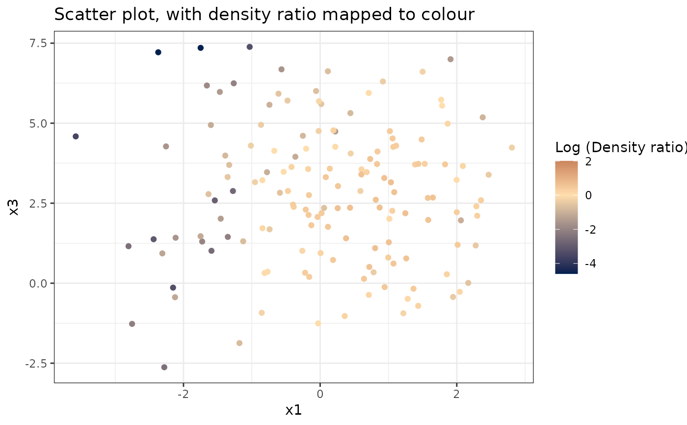
# Plot density ratio for each pair of variables
plot_bivariate(dr)
#> Warning: Negative estimated density ratios for 7 observation(s) converted to 0.01 before applying logarithmic transformation
#> [[1]]
 #>
#> [[2]]
#>
#> [[2]]
 #>
#> [[3]]
#>
#> [[3]]
 #>
# Predict density ratio and inspect first 6 predictions
head(predict(dr))
#> , , 1
#>
#> [,1]
#> [1,] 1.637268
#> [2,] 2.230380
#> [3,] 2.147449
#> [4,] 2.302901
#> [5,] 1.228723
#> [6,] 1.785768
#>
# Fit model with custom parameters
ulsif(numerator_small, denominator_small, sigma = 2, lambda = 2)
#>
#> Call:
#> ulsif(df_numerator = numerator_small, df_denominator = denominator_small, sigma = 2, lambda = 2)
#>
#> Kernel Information:
#> Kernel type: Gaussian with L2 norm distances
#> Number of kernels: 150
#> sigma: num 2
#>
#> Regularization parameter (lambda): num 2
#>
#> Optimal sigma (loocv): 2
#> Optimal lambda (loocv): 2
#> Optimal kernel weights (loocv): num [1:150] 0.0353 0.0558 0.0534 0.0622 0.0111 ...
#>
#>
# Predict density ratio and inspect first 6 predictions
head(predict(dr))
#> , , 1
#>
#> [,1]
#> [1,] 1.637268
#> [2,] 2.230380
#> [3,] 2.147449
#> [4,] 2.302901
#> [5,] 1.228723
#> [6,] 1.785768
#>
# Fit model with custom parameters
ulsif(numerator_small, denominator_small, sigma = 2, lambda = 2)
#>
#> Call:
#> ulsif(df_numerator = numerator_small, df_denominator = denominator_small, sigma = 2, lambda = 2)
#>
#> Kernel Information:
#> Kernel type: Gaussian with L2 norm distances
#> Number of kernels: 150
#> sigma: num 2
#>
#> Regularization parameter (lambda): num 2
#>
#> Optimal sigma (loocv): 2
#> Optimal lambda (loocv): 2
#> Optimal kernel weights (loocv): num [1:150] 0.0353 0.0558 0.0534 0.0622 0.0111 ...
#>