Obtain predicted density ratio values from a kliep object

Obtain predicted density ratio values from a kliep object

Usage

# S3 method for class 'kliep'
predict(object, newdata = NULL, sigma = c("sigmaopt", "all"), ...)

Arguments

object

A kliep object

newdata

Optional matrix new data set to compute the density

sigma

A scalar with the Gaussian kernel width

...

Additional arguments to be passed to the function

Value

An array with predicted density ratio values from possibly new data, but otherwise the numerator samples.

See also

predict, kliep

Examples

set.seed(123)
# Fit model
dr <- kliep(numerator_small, denominator_small)
# Inspect model object
dr
#> 
#> Call:
#> kliep(df_numerator = numerator_small, df_denominator = denominator_small)
#> 
#> Kernel Information:
#>   Kernel type: Gaussian with L2 norm distances
#>   Number of kernels: 150
#>   sigma: num [1:10] 0.711 1.08 1.333 1.538 1.742 ...
#> 
#> Optimal sigma (5-fold cv): 0.7105
#> Optimal kernel weights (5-fold cv):  num [1:150, 1] 0.476 0.67 0.578 0.678 0.603 ...
#> 
#> Optimization parameters:
#>   Learning rate (epsilon): 1e+01  1e+00  1e-01  1e-02  1e-03  1e-04  1e-05
#>   Maximum number of iterations:  5000
# Obtain summary of model object
summary(dr)
#> 
#> Call:
#> kliep(df_numerator = numerator_small, df_denominator = denominator_small)
#> 
#> Kernel Information:
#>   Kernel type: Gaussian with L2 norm distances
#>   Number of kernels: 150
#> Optimal sigma: 0.7105233
#> Optimal kernel weights: num [1:150, 1] 0.476 0.67 0.578 0.678 0.603 ...
#>  
#> Kullback-Leibler divergence between P(nu) and P(de): 0.8268
#> For a two-sample homogeneity test, use 'summary(x, test = TRUE)'.
#> 
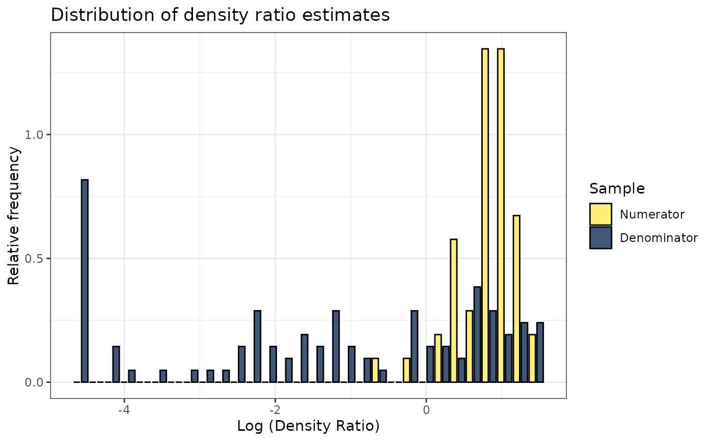
# Plot model object
plot(dr)
#> Warning: Negative estimated density ratios for 16 observation(s) converted to 0.01 before applying logarithmic transformation
#> `stat_bin()` using `bins = 30`. Pick better value with `binwidth`.

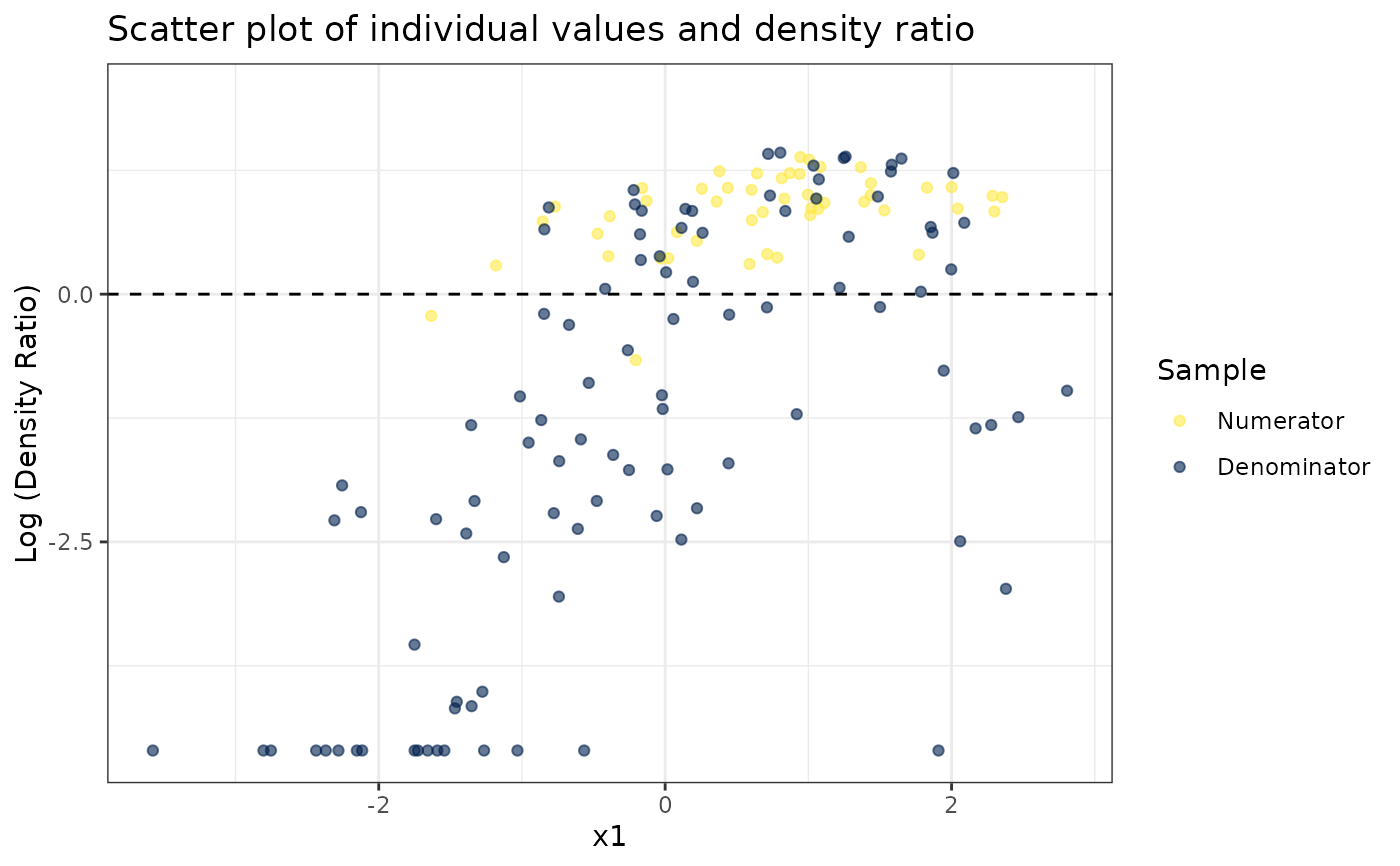
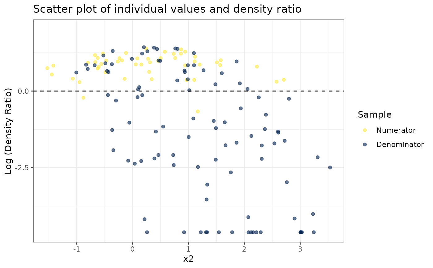
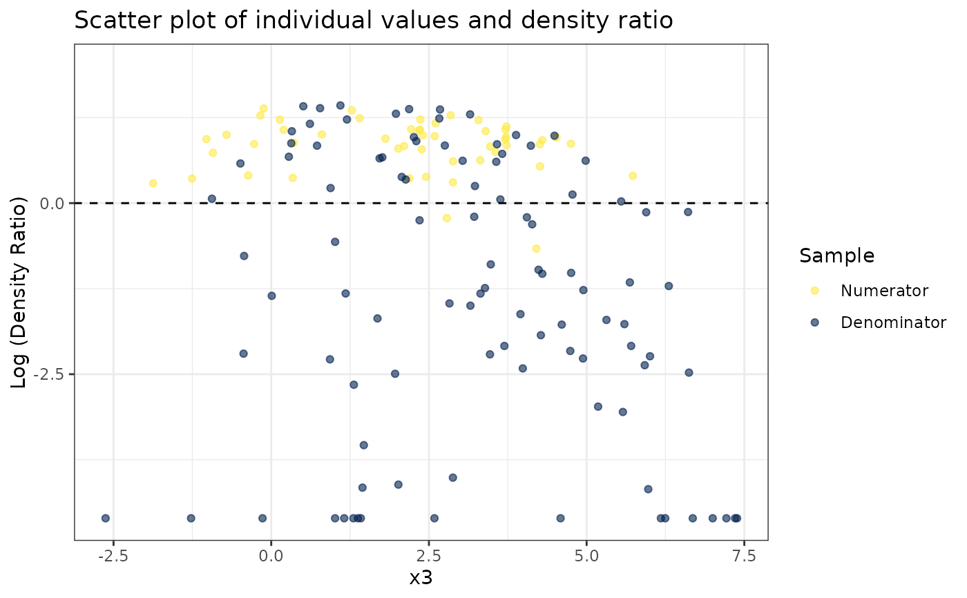
# Plot density ratio for each variable individually
plot_univariate(dr)
#> Warning: Negative estimated density ratios for 16 observation(s) converted to 0.01 before applying logarithmic transformation
#> [[1]]

#> 
#> [[2]]

#> 
#> [[3]]

#> 
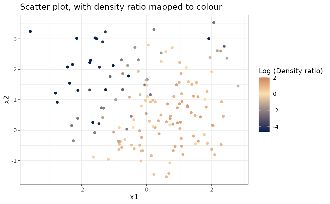
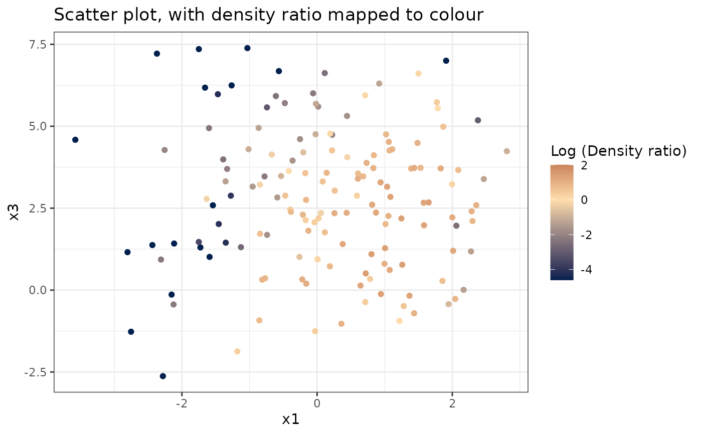
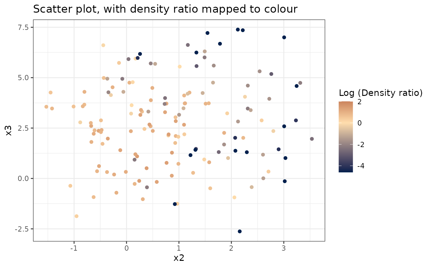
# Plot density ratio for each pair of variables
plot_bivariate(dr)
#> Warning: Negative estimated density ratios for 16 observation(s) converted to 0.01 before applying logarithmic transformation
#> [[1]]

#> 
#> [[2]]

#> 
#> [[3]]

#> 
# Predict density ratio and inspect first 6 predictions
head(predict(dr))
#>          [,1]
#> [1,] 1.432706
#> [2,] 2.696996
#> [3,] 3.600185
#> [4,] 2.715088
#> [5,] 2.219022
#> [6,] 2.930002
# Fit model with custom parameters
kliep(numerator_small, denominator_small,
      nsigma = 1, ncenters = 100, nfold = 10,
      epsilon = 10^{2:-5}, maxit = 500)
#> 
#> Call:
#> kliep(df_numerator = numerator_small, df_denominator = denominator_small,     nsigma = 1, ncenters = 100, nfold = 10, epsilon = 10^{        2:-5    }, maxit = 500)
#> 
#> Kernel Information:
#>   Kernel type: Gaussian with L2 norm distances
#>   Number of kernels: 100
#>   sigma: num 1.85
#> 
#> Optimal sigma (10-fold cv): 1.852
#> Optimal kernel weights (10-fold cv):  num [1:100, 1] 0.039 0 0.0659 0 0.0786 ...
#> 
#> Optimization parameters:
#>   Learning rate (epsilon): 1e+02  1e+01  1e+00  1e-01  1e-02  1e-03  1e-04  1e-05
#>   Maximum number of iterations:  500