Prediction intervals with missing data

Department of Methodology and Statistics, Utrecht University

Thom B. Volker

Florian D. van Leeuwen

Stef van Buuren

Uncertainty quantification

Proper uncertainty quantification is essential in prediction settings

• Expected grade
• Election polling
• Package delivery

Prediction interval

A range of values \([\hat y_l, \hat y_u]\) that cover the true value \(y\) of unseen cases with probability \(1-\alpha\)

Missing data complicates prediction

How to deal with observed predictors?

• Complete case analysis? No.
• Imputation: single (deterministic) or multiple (stochastic)?
  • Single imputation: unbiased predictions (Little 1992), but invalid uncertainty quantification (Van Buuren 2018; Zaffran et al. 2024).
  • Multiple imputation: valid for inference, but how to use for prediction uncertainty?

Calculating prediction intervals

Prediction uncertainty¹

\(U =\) Residual variance + model uncertainty

1. Under standard linear regression assumptions, the prediction interval covers the true \(y\) value with probability \(1-\alpha\).

With missing data

Additional assumption: imputation model is appropriate

Prediction uncertainty with missing data¹

Residual variance + model uncertainty + imputation uncertainty²

1. Under standard linear regression assumptions, plus the assumption that the imputation model is appropriate, the prediction interval covers the true \(y\) value with probability \(1-\alpha\).

2. Obtainable via Rubin’s Rules (1976): \(T = U + B(1 + 1/m)\), \(U =\) residual variance + model uncertainty; \(B(1+1/m) =\) imputation uncertainty.

Evaluation (simulation)

Linear regression model: \(y = X\beta + \varepsilon\)

---

\(X \sim MVN(0, \Sigma)\)

---

MAR missingness in train, test or both

---

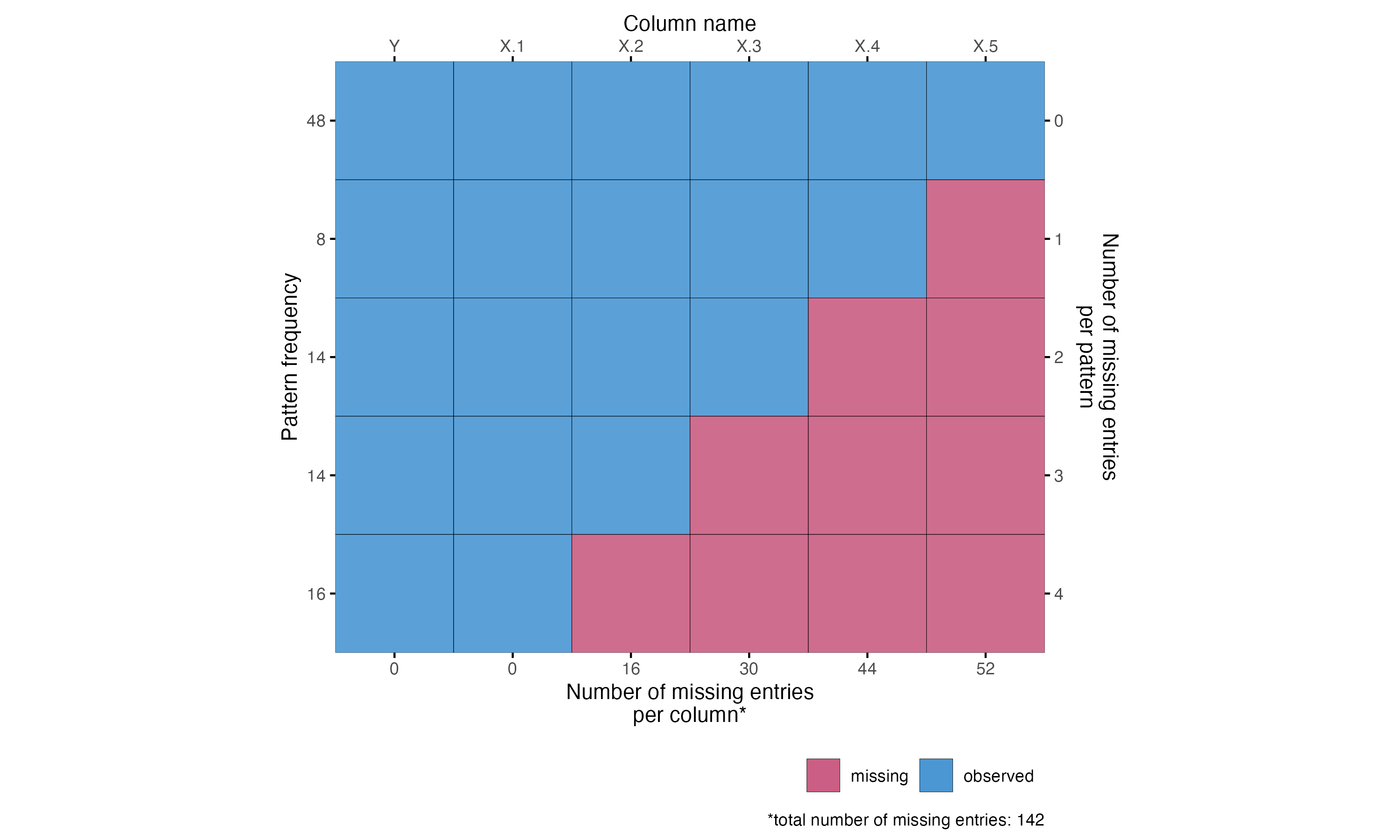
Varied sample size, correlation

Marginal coverage results

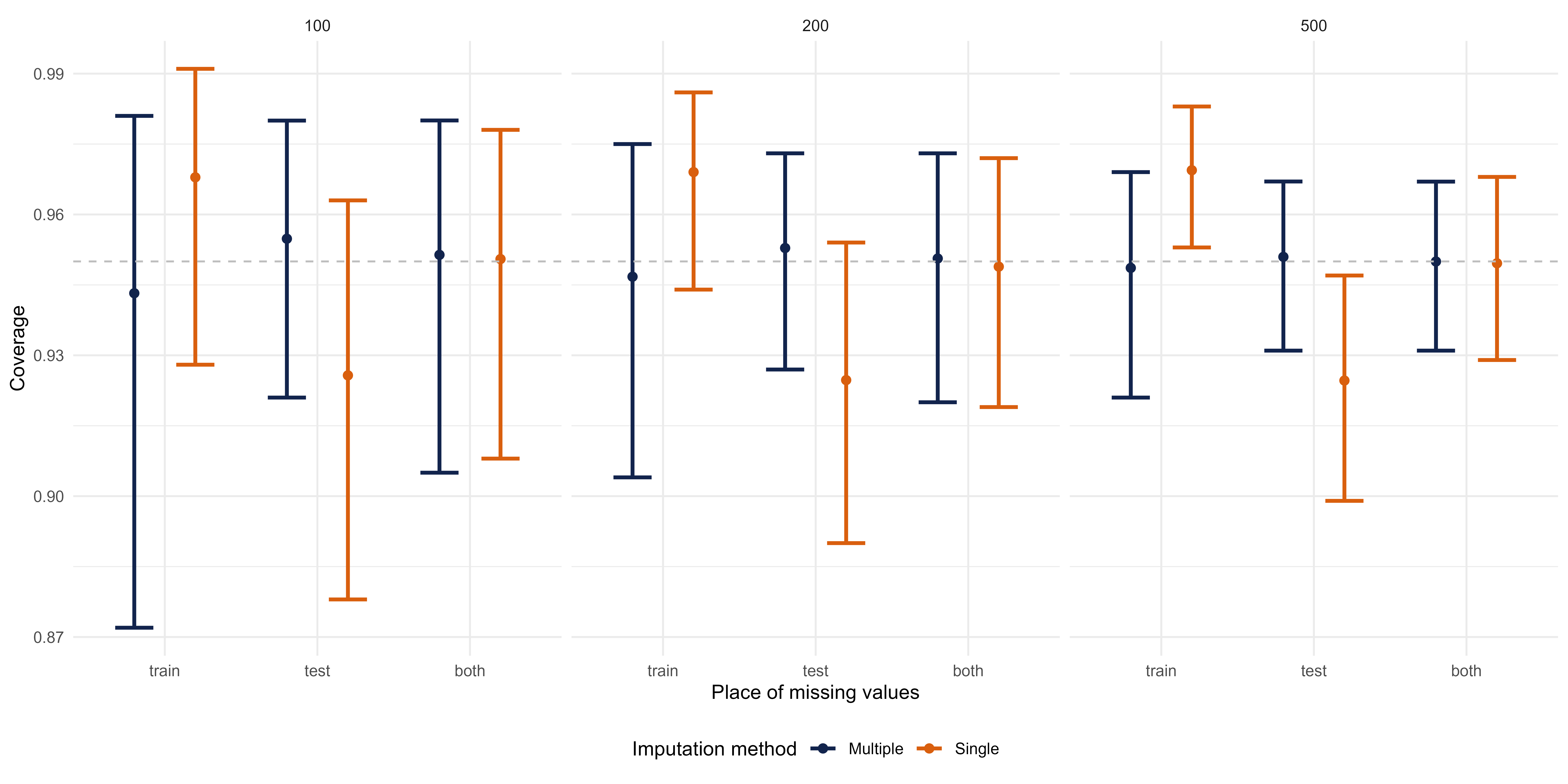
Marginal coverage (y-axis) for multiple and single imputation, depending on whether missingness occurs only in the training data, only in the test data, or in both, for different sizes of the training data.

Conditional coverage results

Conditional coverage (y-axis) for multiple and single imputation, per number of missing observations per record.

Conditional PI width (y-axis) for multiple and single imputation, per number of missing observations per record.

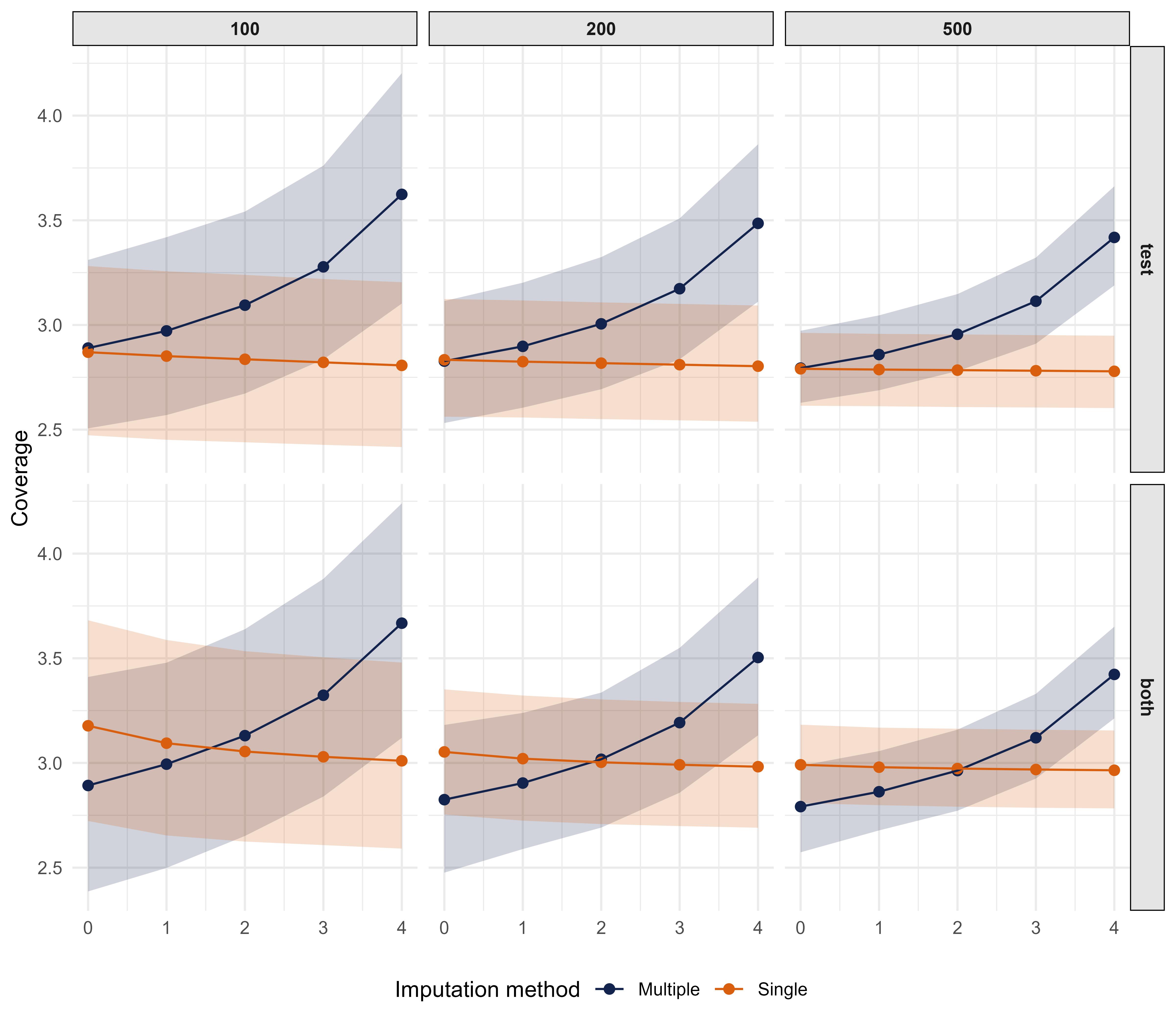
Multiple imputation produces prediction intervals that yield nominal coverage and scale with imputation uncertainty.

• The approach is readily available in the mice package.

• Other (conformal) approaches (e.g., Zaffran et al. 2023, 2024) assume MCAR and require very large samples.

• More research is needed to test our method beyond linear regression.

References

Barnard, J, and DB Rubin. 1999. “Small-Sample Degrees of Freedom with Multiple Imputation.” Biometrika 86 (4): 948–55. https://doi.org/10.1093/biomet/86.4.948.

Little, Roderick J. A. 1992. “Regression with Missing x ’s: A Review.” Journal of the American Statistical Association 87 (420): 1227–37. https://doi.org/10.1080/01621459.1992.10476282.

Rubin, Donald B. 1976. “Inference and Missing Data.” Biometrika 63 (3): 581–92. https://academic.oup.com/biomet/article-abstract/63/3/581/270932.

Van Buuren, Stef. 2018. Flexible Imputation of Missing Data. CRC press. https://books.google.com/books?hl=nl&lr=&id=lzb3DwAAQBAJ&oi=fnd&pg=PP1&dq=Flexible+Imputation+of+Missing+Data&ots=Vh2U_JhbX-&sig=Cv43tBLqwOf6_AMbIK-XHhSTV0k.

Zaffran, Margaux, Aymeric Dieuleveut, Julie Josse, and Yaniv Romano. 2023. “Conformal Prediction with Missing Values.” In Proceedings of the 40th International Conference on Machine Learning, 40578–604. PMLR. https://proceedings.mlr.press/v202/zaffran23a.html.

Zaffran, Margaux, Julie Josse, Yaniv Romano, and Aymeric Dieuleveut. 2024. “Predictive Uncertainty Quantification with Missing Covariates.” arXiv. https://doi.org/10.48550/arXiv.2405.15641.

Prediction interval calculation

Standard linear model prediction variance \[ U = \hat \sigma^2 (1 + x^T (X^TX)^{-1} x) \] and prediction interval \[ [\hat y - t_{\alpha/2, n-p}\sqrt U, \hat y + t_{\alpha/2, n-p}\sqrt U], \] based on a \(t\)-distribution with \(n - p\) degrees of freedom.

Prediction intervals with missing data

With missing data, the prediction variance equals \[ T = \bar U + B(1 + 1/m), \] with \(B = \text{var} [\hat y_j]\) over imputations \(j = 1, \dots, m\). The prediction interval equals \[ [\bar {\hat y}_j - t_{\alpha/2, \nu}\sqrt T, \bar {\hat y}_j + t_{\alpha/2, \nu}\sqrt T], \] where \(\bar {\hat y}_j = \sum_j \hat y_j\) and \(\nu\) denotes the missing data degrees of freedom (Barnard and Rubin 1999).