Today, I was doing some programming for the R software mice, and it turns out I needed to calculate the residual degrees of freedom after performing regression with a ridge penalty to improve numerical stability. Perhaps, I thought, the glmnet package might provide any help, and at least may serve to verify my understanding. Although I love the glmnet package, I should’ve known better. That is, the package is great for estimation, but makes some design choices that are buried somewhere deep in the documentation, which can make it hard to find what is actually going on under the hood. In the end, I found out how glmnet performs ridge regression, so all good, I suppose.
Ridge regression
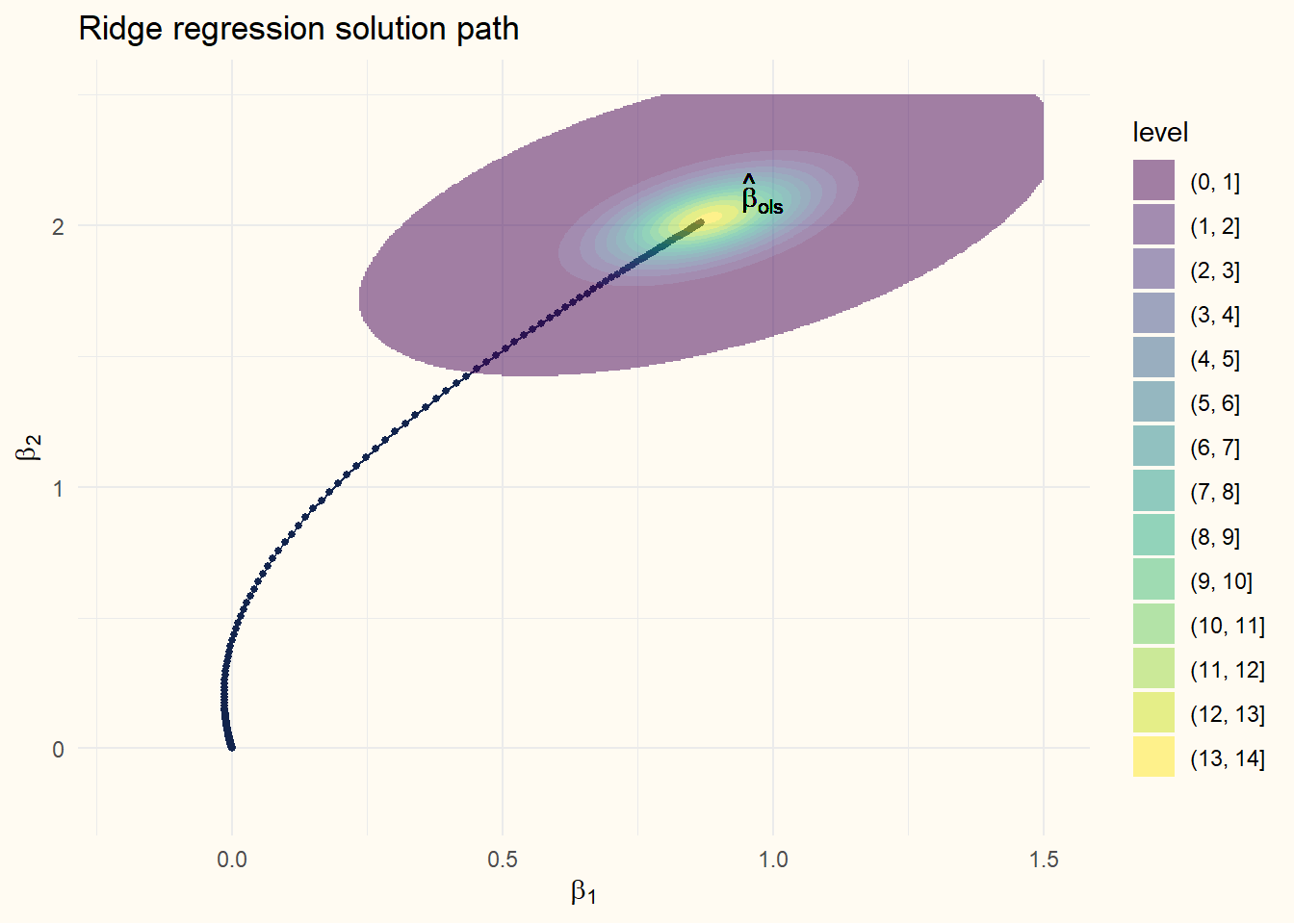
Ridge regression is a regression technique that is highly useful when there are relatively many predictors, or when predictors are highly correlated (i.e., when the \(n \times p\) predictor matrix \(X\) is (close to) rank deficient). In such instances, the usual least-squares solution \(\hat\beta = (X'X)^{-1}X'y\) may have very large variance, and may be impossible to compute. In such instances, adding a positive penalty to the diagonal of the crossproduct of the predictor matrix ensures invertibility and reduces the variance of the resulting estimates. An alternative way to think about this penalty is as a penalty on this size of the regression coefficients. The larger this penalty, the closer the coefficients will be to zero. Hence, ridge regression can be considered a compromise between the least-squares solution and a solution that shrinks all coefficients towards zero.
The ridge regression problem is commonly denoted as \[
\min_\beta \left\{ ||y - \beta_0 - X\beta||_2^2 + \lambda ||\beta||_2^2 \right\},
\] where \(||\cdot||_2\) denotes the \(\ell_2\) norm, \(y\) is the response vector, \(\beta_0\) denotes an intercept, \(\beta\) denotes the regression coefficients and \(\lambda\) is a positive hyperparameter that controls the amount of shrinkage. First, we make explicit that the intercept term \(\beta_0\) is typically not penalized, because it simply denotes the conditional mean of \(y\) if all predictors are zero. It is not hard to see that when \(\lambda = 0\), the problem reduces to the least-squares problem, and when \(\lambda \to \infty\), the penalty dominates the fit of the model, and \(\beta \to 0\).
For now, we ignore the intercept, and denote \(\tilde y = y - \beta_0\). To minimize the objective \[
\left\{ ||\tilde y - X\beta||_2^2 + \lambda ||\beta||_2^2 \right\}
\] we expand it as \[
\min_\beta \left\{ \tilde y^T\tilde y - 2\tilde y^TX\beta + \beta^TX^TX\beta + \lambda\beta^T\beta \right\},
\] using the inner product \(||a||_2^2 = a^Ta\), where \(T\) denotes the transpose operator. To find the optimal parameters, we take the derivative and set it to zero, which yields \[
\begin{aligned}
\nabla_\beta \left\{ \tilde y^T\tilde y - 2\tilde y^TX\beta + \beta^TX^TX\beta + \lambda\beta^T\beta \right\} &= 0 \\
\implies -2X^T\tilde y + 2X^TX\beta + 2\lambda\beta &= 0 \\
\implies (X^TX + \lambda I_p)\beta &= X^T\tilde y \\
\implies (X^TX + \lambda I_p)^{-1}X^T\tilde y &= \beta.
\end{aligned}
\] where \(I_p\) is the \(p \times p\) identity matrix. So far, nothing new under the sun.
Ridge regression with glmnet
To see how glmnet performs ridge regression, we simply use the glmnet function with the alpha = 0 argument.1 Below, we generate a data set of \(n = 200\) observations and \(p=5\) predictors, using variance-covariance matrix \[
V = D\Sigma D,
\] where \(D = \text{diag}(\sqrt 1, \sqrt 2, \dots, \sqrt 10)\) and \(\Sigma\) is a correlation matrix with \(\rho_{ij} = 0.5\) for \(i \neq j\). Moreover, all predictors have mean zero, and the response is generated as \[
y = X\beta + \epsilon,
\] where \(\beta = (0.01, 0.02, \dots, 0.1)^T\) and \(\epsilon \sim N(0, I_n\sigma^2)\) with \(\sigma^2 = 1\).
For the sake of exposition, we choose a single \(\lambda\) value and fix it to \(1.5\), although we would normally use a more principled approach to select an optimal value for \(\lambda\) (e.g., cross-validation). Then, we can proceed the fit the model using glmnet. To keep it simple initially, we don’t estimate an intercept, nor do we standardize the predictors.
library(glmnet)lambda <-1.5fit <-glmnet(x = X, y = y, alpha =0, lambda = lambda, standardize =FALSE, intercept =FALSE)glmnet_coefs <-coef(fit)[,1]round(glmnet_coefs, 3)
The question then is: how can we obtain the same estimates without using the glmnet function. The optimization problem is clear enough, so this should be doable. Let’s try a first naive approach.
D <- lambda *diag(P)b <-solve(crossprod(X) + D, crossprod(X, y))round(b, 3)
Well, clearly, the coefficients are not the same. Typically, they are somewhat larger than the glmnet estimates, although this doesn’t hold for each coefficient. Well, okay, this was a bit stupid, because while my formulation above minimizes the penalized sum of squares, the glmnet function minimizes the penalized mean squared error. To account for this adjustment, we can multiple our penalty parameter with the sample size. Still, if we would make this modification, solely adjusting the penalty term won’t suffice, because glmnet also assumes \(y\) to have unit variance (using the biased variance estimator). Since we don’t estimate an intercept, we can suffice by multiplying the mean squared error by the standard deviation of \(y\), or, equivalently, divide our penalty parameter by the standard deviation of \(y\). Hence, instead of minimizing \[
\left\{ ||y - X\beta||_2^2 + \lambda ||\beta||_2^2 \right\},
\] we should minimize \[
\left\{||y - X\beta||_2^2 + \frac{N}{\sigma_y} \lambda ||\beta||_2^2 \right\}.
\]
Now all coefficients are correct up to the same three decimals. Note that glmnet uses some numerical optimization scheme. Increasing the estimation precision yields almost identical coefficients.
coefs_precise <-glmnet(x = X, y = y, alpha =0, lambda = lambda, standardize =FALSE, intercept =FALSE,thres =1e-16,maxit =999999999) |>coef()coefs_precise[2:11] - b
So, taking some shortcuts, we can obtain the same estimates as glmnet. Now, let’s see if we can get the same estimates without taking any shortcuts (fortunately, we can, because otherwise I wouldn’t have written this up).
Before proceeding, let’s estimate the ridge regression coefficients with glmnet using all default settings.
default_fit <-glmnet(x = X, y = y, alpha =0, lambda = lambda)coef(default_fit)[,1]
By now, we know that glmnet standardizes predictors and outcomes, so let’s start from there. However, when estimating the coefficients on the standardized data, we need to backtransform the coefficients to the original scale.
Hooray! The coefficients look very similar to the glmnet coefficients. But wait.. We are missing the intercept still. Fortunately, it is not too hard to add the intercept back in. Recall that the intercept is simply the expected value of \(y\) when all predictors are equal to zero. By centering each predictor, this corresponds to the expected value of \(y\) when all predictors are equal to their mean. So, we can obtain the intercept by taking the mean of \(y\) and subtract the mean of each predictor multiplied with the respective regression coefficient.
b0 <-mean(y) -colMeans(X) %*% b
To finish it off, we can estimate the glmnet model with larger precision again, and compare our estimates.
fit <-glmnet(x = X, y = y, alpha =0, lambda = lambda, standardize =TRUE, intercept =TRUE,maxit =999999999,thresh =1e-16)coef(fit)[,1] -c(b0, b)
By default, glmnet fits a lasso regression model, which is fairly similar but uses an \(\ell_1\) penalty for the coefficients, which results in some coefficients estimated to be precisely zero. Changing the alpha parameter yields a mixture between 1-alpha times the ridge penalty and alpha times the lasso penalty.↩︎