We consider the case of a one-sample \(t\)-test. To fix notation, let \(X_1, \ldots, X_n\) be a sample of size \(n\) from a normal distribution with unknown mean \(\mu\) and unknown variance \(\sigma^2\). We are interested in testing the null hypothesis \(H_0: \mu = \mu_0\) against the alternative hypothesis \(H_1: \mu \neq \mu_0\). Moreover, we use the approximate adjusted fractional Bayes factor (AAFBF; Gu, Mulder & Hoijtink, 2017), which implies that we approximate the posterior distribution of the parameters by a normal distribution with mean and variance equal to the (unbiased) maximum likelihood estimates. Using this method, the Bayes factor is given by \[
\begin{aligned}
BF_{0,u} &= \frac{f_0}{c_0} \\
&= \frac{P(\mu = \mu_0 | X, \pi_0)}{P(\mu = \mu_0 | \pi_0)},
\end{aligned}
\] where \(f_0\) denotes the fit of the posterior to the hypothesis of interest, \(c_0\) denotes the complexity of the hypothesis of interest, \(X\) denotes the data, and \(\pi_0\) denotes the prior distribution of the parameters under the null hypothesis. Given our normal approximation and the definition of the fractional adjusted Bayes factor, the prior is given by \[
\pi_0 = \mathcal{N}
\Big(\mu_0, \frac{1}{b} \frac{\hat{\sigma}^2}{n}\Big),
\] where \(b\) is the fraction of information in the data used to specify the prior distribution, typically specified as \(J/n\), and \(\hat{\sigma}^2\) is the unbiased estimate of the variance of the data. For the one-sample \(t\)-test, we set \(J=1\) and thus \(b = \frac{1}{n}\), such that we have \[
\pi_0 = \mathcal{N}(\mu_0, \hat{\sigma}^2).
\] Additionally, the posterior distribution is given by \[
\pi = \mathcal{N}\Big(\hat{\mu}, \frac{\hat{\sigma}^2}{n}\Big).
\] Without loss of generality, we can rescale the data by subtracting the hypothesized mean and dividing by the standard error \(\frac{\hat{\sigma}}{\sqrt{n}}\), such that we have \[
\begin{aligned}
\pi_0 &= \mathcal{N}(0, n), \\
\pi &= \mathcal{N}(\tilde{\mu}, 1),
\end{aligned}
\] where \(\tilde{\mu} = \frac{\hat{\mu} - \mu_0}{\hat{\sigma}/\sqrt{n}}\).
To show this, consider the following example, where we have a sample of size \(n = 20\) drawn from a normal distribution with mean \(\mu = 0\) and standard deviation \(\sigma = 1\). We are interested in testing the null hypothesis \(H_0: \mu = 0\) against the alternative hypothesis \(H_1: \mu \neq 0\).
Bayesian informative hypothesis testing for an object of class t_test:

   Fit   Com   BF.u  BF.c  PMPa  PMPb  PMPc
H1 1.484 0.410 3.618 3.618 1.000 0.783 0.783
Hu                               0.217
Hc                                     0.217

Hypotheses:
  H1: x=0

Note: BF.u denotes the Bayes factor of the hypothesis at hand versus the unconstrained hypothesis Hu. BF.c denotes the Bayes factor of the hypothesis at hand versus its complement. PMPa contains the posterior model probabilities of the hypotheses specified. PMPb adds Hu, the unconstrained hypothesis. PMPc adds Hc, the complement of the union of the hypotheses specified.
f0 <-1/sqrt(2* pi * sdx^2/ n) *exp(-mux^2/ (2* sdx^2/ n))c0 <-1/sqrt(2* pi * sdx^2/J) *exp(-0^2/ (2* sdx^2/J))f0 / c0
[1] 3.617783
# of course, we can also make use of the in-build functionalitydnorm(mux, 0, sdx /sqrt(n)) /dnorm(0, 0, sdx/J)
[1] 3.617783
Alternatively, we can use the simplified expression like so.
It is easy see that the Bayes factor is only a function of the scaled sample mean.
Power of a Bayesian one-sided t-test by simulation
To obtain the power of a test with sample size \(n\), we need to calculate the probability that the Bayes factor is larger than a certain value \(Q\). To do this we generate nsim = 100000000 samples of size \(n\) from a normal distribution, calculate the Bayes factor for the null hypothesis \(\mu = 0\) against the unconstrained alternative hypothesis, and calculate how often the Bayes factor exceeds the critical value \(T\). For now, suppose \(Q = 3\).
library(pbapply)nsim <-10000000Q <-3n <-20mu <-0sd <-1mu0 <-0simfunc <-function(n =20, mu =0, sd =1, J =1, mu0 =0) { x <-rnorm(n, mu, sd) mu <-mean(x) se <-sqrt(var(x)/n) mutilde <- (mu - mu0) / se BF <-sqrt(n/J) *exp(-mutilde^2/2) BF}pboptions(type ="timer")cl <- parallel::makeCluster(16)parallel::clusterExport(cl, c("simfunc", "n", "mu", "sd", "J", "mu0"))bfs <-pbreplicate(nsim, simfunc(n = n, mu = mu, sd = sd, mu0 = mu0), cl = cl)parallel::stopCluster(cl)mean(bfs > Q)
[1] 0.6171808
Hence, the power of the test is approximately \(0.617\).
Power of a Bayesian one-sided t-test by analytical calculation
Now, noting that the Bayes factor only depends on the scaled sample mean, we can calculate the power analytically. Importantly, note that the distribution of the scaled sample mean with unknown variance follows a non-central \(t\)-distribution with \(n-1\) degrees of freedom, and non-centrality parameter \(\delta = (\mu - \mu_0) / (\sigma/\sqrt{n})\). This scaling of the non-centrality parameter arises because we center the data to the hypothesized value and scale by it’s standard error. Therefore, we have to apply the same scaling to the population mean \(\mu\). If the variance was known, the distribution would be a normal distribution with mean \(\mu / (\sigma/\sqrt{n})\) and standard deviation \(1\).
The next step is to calculate for which values of \(\tilde{\mu}\) the Bayes factor exceeds the threshold \(Q\). Per Equation 1, we have that \[
\begin{aligned}
Q &\leq \sqrt{n} \exp \Big\{-\frac{\tilde{\mu}^2}{2} \Big\} \\
\frac{Q}{\sqrt{n}} &\leq \exp \Big\{-\frac{\tilde{\mu}^2}{2} \Big\} \\
\log \Big(\frac{Q}{\sqrt{n}} \Big) &\leq -\frac{\tilde{\mu}^2}{2} \\
2 \log \Big(\frac{\sqrt{n}}{Q} \Big) &\leq \tilde{\mu}^2 \\
\tilde\mu &\in \Bigg[-\sqrt{2 \log \Big(\frac{\sqrt{n}}{Q} \Big)}, \sqrt{2 \log \Big(\frac{\sqrt{n}}{Q} \Big)}\Bigg].
\end{aligned}
\] Hence, as long as \(\tilde\mu\) falls within the interval \(\Big[-\sqrt{2 \log \Big(\frac{\sqrt{n}}{Q} \Big)}, \sqrt{2 \log \Big(\frac{\sqrt{n}}{Q} \Big)}\Big]\), the Bayes factor will exceed the threshold \(Q\).
The final step is to calculate the probability with which the scaled sample mean falls within this interval. This can be done by calculating the cumulative distribution function of the non-central \(t\)-distribution with \(n-1\) degrees of freedom and non-centrality parameter \(\delta = \mu / (\sigma/\sqrt{n})\) at the upper and lower bounds of the interval defined by \(\mu_\text{critical}\).
In case the distribution of the statistic of interest is not known exactly, but can be approximated by a normal distribution, we can also use the cumulative normal distribution function. Note that this would not alter the critical value of the sample mean \(\mu_\text{critical}\), but solely alters the sampling distribution of the mean. In this case, we would have that the scaled sample mean follows a normal distribution with mean \(\mu / (\sigma/\sqrt{n})\) and standard deviation \(1\).
So far, we assumed that \(J = 1\), and thus the fraction of information used in the training data equals \(b = \frac{1}{n}\). However, using a different value for \(J\) would yield a different Bayes factor value. Hence, this value alters the calculation of the critical value \(Q\), but not the sampling distribution of the mean. Moreover, the value of \(J\) only alters the prior distribution, which then yields \[
\pi_0 = \mathcal{N}
\Big(\mu_0, \frac{\hat{\sigma}^2}{J}\Big).
\] Accordingly, the Bayes factor equals \[
\begin{aligned}
BF_{0,u} &= \frac{
\frac{1}{\sqrt{2\pi\frac{\hat{\sigma}^2}{n}}}
\exp \Big\{-\frac{(\hat{\mu} - \mu_0)^2}{2\frac{\hat{\sigma}^2}{n}} \Big\}
}{
\frac{1}{\sqrt{2\pi\hat{\sigma}^2/J}}
\exp \Big\{-\frac{(\mu_0-\mu_0)^2}{2\frac{\hat{\sigma}^2}{J}} \Big\}
} \\
&= \frac{
\frac{1}{\sqrt{2\pi}} \exp \Big\{-\frac{\tilde{\mu}^2}{2} \Big\}
}{
\frac{1}{\sqrt{2\pi \frac{n}{J}}}
} \\
&= \sqrt{\frac{n}{J}} \exp \Big\{-\frac{\tilde{\mu}^2}{2} \Big\},
\end{aligned}
\tag{2}\] and we can define the critical value of the scaled sample mean as \(\mu_\text{critical}\) for which the Bayes factor exceeds \(Q\) as \[
\begin{aligned}
Q &\leq \sqrt{\frac{n}{J}} \exp \Big\{-\frac{\tilde{\mu}^2}{2} \Big\} \\
\frac{Q}{\sqrt{n/J}} &\leq \exp \Big\{-\frac{\tilde{\mu}^2}{2} \Big\} \\
\log \Big(\frac{Q}{\sqrt{n/J}} \Big) &\leq -\frac{\tilde{\mu}^2}{2} \\
2 \log \Big(\frac{\sqrt{n/J}}{Q} \Big) &\leq \tilde{\mu}^2 \\
\tilde\mu &\in \Bigg[-\sqrt{2 \log \Big(\frac{\sqrt{n/J}}{Q} \Big)}, \sqrt{2 \log \Big(\frac{\sqrt{n/J}}{Q} \Big)}\Bigg].
\end{aligned}
\]
Examples
The BFpower function
Compiling the above equations in a single R function yields the following code.
Increasing \(J\), we put a more informative prior on the parameter of interest. Accordingly, the Bayes factor in favor of the null hypothesis decreases. This is because the prior distribution is more concentrated around the null hypothesis, and thus the data are more likely to provide evidence against the null hypothesis compared to our a priori beliefs.
To evaluate the power of an informative hypothesis against the unconstrained hypothesis, we can use a similar approach. However, if the informative hypothesis of interest is an inequality-constrained hypothesis, the Bayes factor is defined in a slightly different way. In this case, we can make use of the encompassing prior approach put forward by Klugkist et al. (2005). Under this set-up, the Bayes factor for the inequality-constrained hypothesis evaluated against the unconstrained hypothesis is given by \[
\begin{aligned}
BF_{i,u} &= \frac{f_i}{c_i} \\
&=
\frac{
\int_{\mu \in M_i} \pi(\mu|X)
}{
\int_{\mu \in M_i} \pi_0(\mu)
},
\end{aligned}
\] where \(M_i\) denotes the parameter space under the inequality-constrained hypothesis, \(\pi(\mu|X)\) denotes the posterior distribution of the mean given the data (marginalized over the variance), and \(\pi_0(\mu)\) denotes the prior distribution of the mean (also marginalized over the variance).
Bayesian one-sided hypothesis evaluation
First, assume that the hypothesis of interest is a one-sided hypothesis, in the sense that we consider \(H_i: \mu > \mu_0\) or \(H_{i'}: \mu < \mu_0\). In this setting, centering the prior distribution at the hypothesized value yields a complexity of \(c_i = 0.5\), and thus we have that \(BF_{i,u} = 2 \cdot f_i\). From this observation, it follows that the maximum Bayes factor equals \(BF_{i,u}^\max=2\), whereas the minimum Bayes factor equals \(BF_{i,u}^\min=0\). Moreover, since a normal approximation is used to the posterior distribution of the parameters, we have that \[
\begin{aligned}
BF_{i,u} &= 2 \int_{\mu \in M_i}
\frac{1}{\sqrt{2\pi \frac{\hat\sigma^2}{n}}}
\exp \Big\{ -\frac{(\hat\mu - \mu_0)^2}{2 \frac{\hat\sigma^2}{n}} \Big\} d\mu,\\
&= 2 \int_{\mu \in M_i} \frac{1}{\sqrt{2 \pi}} \exp \Big\{ -\frac{\tilde\mu^2}{2} \Big\} d\mu,\\
&= 2 \cdot (\Phi(\sup(M_i)) - \Phi(\inf(M_i))),
\end{aligned}
\] where \(\Phi\) denotes the cumulative distribution function of the normal distribution with mean \(\tilde\mu\) and variance \(1\), and \(\sup(M_i)\) and \(\inf(M_i)\) denote the upper and lower bounds of the parameter space under the inequality-constrained hypothesis, respectively. Assuming that the hypothesis of interest is \(H_i: \mu > x\) or \(H_{i'}: \mu < x\), with the prior distribution centered at \(x\), we either have that \(\Phi(\sup(M_i)) = 1\) or \(\Phi(\inf(M_i)) = 0\), respectively. Hence, the critical value for \(\tilde\mu\) that corresponds to a Bayes factor of \(Q\) is given by \[
\begin{aligned}
\mu_\text{critical} = \pm \Phi^{-1}(Q/2),
\end{aligned}
\] where the \(\pm\) sign depends on whether the hypothesis of interest is \(H_i\) or \(H_{i'}\) and \(\Phi^{-1}\) denotes the inverse of the cumulative normal distribution. The next step is to obtain the power by quantifying the probability that Accordingly, the power of the test is given by the probability that \(\tilde\mu > \mu_\text{critical}\). Again, this probability is given by the cumulative distribution function of the non-central \(t\)-distribution with \(n-1\) degrees of freedom and non-centrality parameter \(\delta = (\mu-\mu_0)/(\sigma^2/n)\).
Bayesian informative hypothesis testing for an object of class t_test:

   Fit   Com   BF.u  BF.c  PMPa  PMPb  PMPc
H1 0.743 0.500 1.485 2.884 1.000 0.598 0.743
Hu                               0.402
Hc 0.257 0.500 0.515                   0.257

Hypotheses:
  H1: x>0

Note: BF.u denotes the Bayes factor of the hypothesis at hand versus the unconstrained hypothesis Hu. BF.c denotes the Bayes factor of the hypothesis at hand versus its complement. PMPa contains the posterior model probabilities of the hypotheses specified. PMPb adds Hu, the unconstrained hypothesis. PMPc adds Hc, the complement of the union of the hypotheses specified.
Using the equations defined above, we can again create a power function for Bayesian one-sided hypothesis evaluation. Note that for these hypotheses, the Bayes factor is defined irrespective of the fraction of information \(J\) used to construct the prior.
We now extend the power calculation to evaluating range hypotheses, in the sense of \(\mu \in [R_l, R_u]\), where \(R_l\) and \(R_u\) denote the lower and upper bound of the range hypothesis. In this case, we assume that the prior distribution is centered around the center of the hypothesis space, such that the prior distribution is symmetric between the bounds of the hypothesis. Note that because the number of independent constraints in this hypothesis equals \(2\), the minimal fraction of information used equals \(\frac{1}{n/J}\), with \(J\) at least equal to \(2\). Accordingly, we can define the prior mean \(\mu_0 = (R_l + R_u)/2\), and calculate the complexity of the hypothesis as \[
c_i = 1 - 2 \cdot\Phi\Big(\frac{R_l - \mu_0}{\sqrt{\hat\sigma^2/J}}\Big).
\] To determine the fit of the hypothesis, we cannot use this symmetry property, because the posterior distribution is not symmetric around the center of the hypothesis space (unless the posterior mean is exactly equal to the posterior mean). Instead, the fit of the hypothesis of interest is calculated as \[
f_i = \Phi\Bigg(\frac{R_u - \hat\mu}{\sqrt{\hat\sigma^2/n}}\Bigg) - \Phi\Bigg(\frac{R_l - \hat\mu}{\sqrt{\hat\sigma^2/n}}\Bigg).
\]
Sketch of the approach to take
Start from the assumption that \(\hat\sigma^2\) is fixed, so that the complexity is determined a priori. Then, we can calculate the maximum Bayes factor that is obtainable (\(1/c_i\)), and we can obtain the probability that \(f_i\) is greater by some value, by calculating how far from the bounds it must be to exceed some value. Say we fix \(\hat\sigma^2 = 1\) and set \(J=2\) and \(R_l = -0.1\) and \(R_u = 0.1\). Then, the complexity is defined as follows.
1-2*pnorm(-0.1, 0, 1/2)
[1] 0.1585194
Moreover, to obtain a Bayes factor of \(Q \geq 2\), the fit of the hypothesis must be at least \(f_i \geq 0.317\). Given that we again fix the variance \(\hat\sigma^2 = 1\) and have \(n = 20\), \(\mu\) must lie between the following numbers to obtain a fit of \(f_i \geq 0.317\).
mu <-0sigma <-1n <-20fi <-function(mu, varx, n, Rl, Ru) {pnorm(Ru, mu, sqrt(varx/n)) -pnorm(Rl, mu, sqrt(varx/n))}D <-uniroot(\(x) fi(x, sigma, n, -0.1, 0.1) -2* (1-2*pnorm(-0.1, 0, sigma/sqrt(2))), interval =c(0, 10000))$root
We can again calculate the probability that \(\hat\mu\) lies between \((R_l + R_u)/2 \pm D\) using a \(t\)-distribution.
bf <-function(meanx, varx, n, J =1, Rl, Ru) { ci <-pnorm(Ru, (Rl+Ru)/2, sqrt(varx/(2*J))) -pnorm(Rl, (Rl+Ru)/2, sqrt(varx/(2*J))) fi <-pnorm(Ru, meanx, sqrt(varx/n)) -pnorm(Rl, meanx, sqrt(varx/n))c(ci = ci, fi = fi, BF = fi/ci)}bf(mean(x), var(x), n, 1, -0.1, 0.1)
       ci        fi        BF
0.1156015 0.2908178 2.5156912
bain::bain(fit, "x > -0.1 & x < 0.1", fraction =1)$fit$BF.u[1]
## But, because we fix the variance here, we can use a normal distribution, ## instead of the t-distributionpnorm(D*sqrt(20)) -pnorm(-D*sqrt(20))
[1] 0.6615538
So, using some simplifying assumptions, it is easy to calculate the power of the hypothesis of interest approximately. Once the variance is known, it is straightforward to calculate the power, also for different variances and sample sizes. However, we now note that not only the mean varies between samples, the estimated variance varies over the samples as well. The estimated variances affect both the complexity and the fit of the hypothesis, and thus introduces an additional complexity, because it affects both in different ways.
A better approximation
To calculate the power of the Bayes factor of an informative hypothesis, we need to calculate the following triple integral \[
\int_{-\infty}^{\infty}\int_0^{\infty}
\mathbb{I}\Bigg\{
\int_{R_l}^{R_u}
\frac{1}{\sqrt{2\pi\hat\sigma^2/n}}
\exp\Big\{-\frac{(x - \hat\mu)^2}{2\hat\sigma^2/n}\Big\} \text{d}x ~~ \Big/ \\
\int_{R_l}^{R_u}\frac{1}{\sqrt{2\pi\hat\sigma^2/J}}
\exp\Big\{-\frac{(x - \mu^*)^2}{2\hat\sigma^2/J}\Big\}
\text{d}x > T \Bigg\}
\text{d}\hat\sigma \text{d}\hat\mu,
\] where \(\mu^*\) is defined as \((R_l * R_u)/2\), \(\mathbb{I}\) denotes the indicator function and \(T\) defines the Bayes factor threshold. Additionally, we assume a normally distributed sample mean \(\hat\mu\) with population mean \(\mu\) and population variance \(\sigma^2/n\) and a scaled chi-squared distributed sample variance \(\hat\sigma^2\) with scaling factor \((n-1)\sigma^2\) and \(n-1\) degrees of freedom (TODO: check whether formulation of variance is correct).
We integrate over the sampling distributions of the mean and the variance. In compact notation, we can rewrite this as \[
\int_{-\infty}^{\infty}\int_0^{\infty} \mathbb{I} \Big\{ f_i(\hat\mu, \hat\sigma, n)/c_i(\hat\sigma, J) > T \Big\}
\text{d}\hat\mu \text{d}\hat\sigma,
\] where we explicitly rewrite the fit and complexity as functions of the mean, variance, sample size and fraction of information used.
Integrating complexity over the variance
We establish that the complexity is a function of the variance only, and it’s threshold is easily calculated using a chi-square distribution. Then, we can easily calculate the boundary value for which the complexity exceeds some threshold, and calculate the probability that the complexity exceeds this boundary value.
Below, we set the variance equal to \(\sigma^2 = 1\) and \(\sigma^2 = 2^2 = 4\) and evaluate the probability that the complexity is smaller than \(0.15\) and \(0.1\), respectively.
## And using variance 1bfs <-sapply(1:1000000, \(i) { x <-rnorm(20)bf(mean(x), var(x), 20, 1, -0.1, 0.1)})mean(bfs[1,] <0.15)
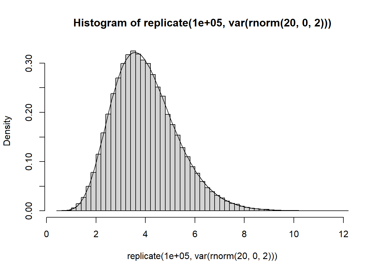
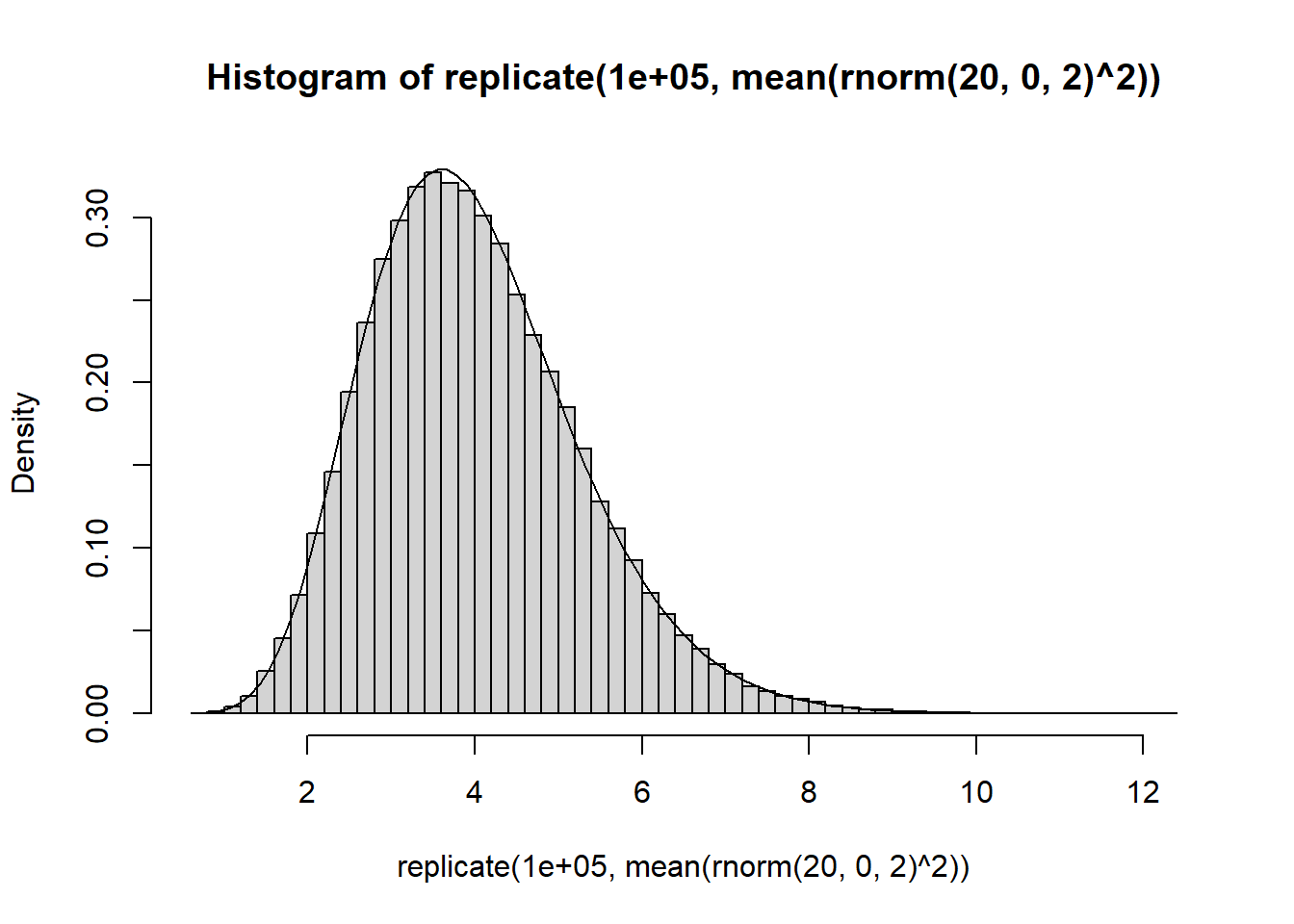
When the mean of the distribution is known, the sampling distribution distribution follows a scaled chi-squared distribution \(\hat\sigma^2 \sim \sigma/n \cdot \chi^2_n\). When the mean of the distribution is unknown, the sampling distribution also follows a chi-squared distribution, but one degree of freedom is lost by calculating the sample mean, which yields \(\hat\sigma^2 \sim \sigma/(n-1) \cdot \chi^2_{n-1}\).
# distribution of the variance:hist(replicate(100000, var(rnorm(20, 0, 2))), freq=FALSE, breaks =50)curve(dchisq(x *19/4, 19) *19/4, add =TRUE)
For the fit of the hypothesis, we also want to calculate the probability that some threshold is exceeded. This is a bit more difficult, because the fit is a function of both the variance and the mean. However, we can automate this using the cubature package, which calculates the integral numerically. To do this, we can define the distribution of the mean and the variance, and integrate the indicator function for the Bayes factors over these distributions.
Unfortunately, this whole set-up is rather slow, perhaps because the indicator function yields a non-smooth function to be evaluated by the integral. To speed this up, we can also approximate the integral using a smooth function approximation to this indicator function, by specifying a steep logit curve at the threshold point, where the function moves quickly from zero to one. An alternative could be to lower the tolerance, but we use this approach first.
This approach shows that we can get a reasonable approximation of the power of the Bayes factor using a smooth approximation to the indicator function. To further speed up the function evaluation, we can also lower the tolerance of the adaptIntegrate() function.
Integrating the Bayes factor over fit and complexity
Now we have everything in place to calculate the power of the Bayes factor over both the fit and complexity of the hypothesis of interest. In fact, we can simply expand the calculation of fit by incorporating the calculation of the complexity as well, which yields the power of the Bayes factor. We made some additional adaptations to the previous code to enhance computational efficiency, for example by vectorizing the computations.
integrand <- \(musigmahat, threshold, mu, var, n) { df <- n-1 dfvar <- df/var sn <-sqrt(musigmahat[2,]/n) s2 <-sqrt(musigmahat[2,]/2) fit <-pnorm(0.1, musigmahat[1,], sn) -pnorm(-0.1, musigmahat[1,], sn) comp <-1-2*pnorm(-0.1, 0, s2) ind <-1/ (1+exp(-1000* (fit/comp - threshold)))matrix(ind *dnorm(musigmahat[1,], mu, sqrt(var/n)) *dchisq(musigmahat[2,]*dfvar, df) * dfvar,ncol =ncol(musigmahat))}system.time( res <-adaptIntegrate( integrand, lower =c(-Inf, 0),upper =c(Inf, Inf),threshold =2, mu =0, var =2, n =20,vectorInterface =TRUE ))
Now we are able to calculate the power of the Bayes factor for a given sample size on the basis of the mean and variance of the data, without having to sample from any distribution.
We can now easily use R’s built-in root-finding algorithm to compute for which sample size the power of the Bayes factor exceeds some threshold.
power <-0.8fx <- \(x) {adaptIntegrate( integrand,lower =c(-Inf, 0),upper =c(Inf, Inf),threshold =2, mu =0, var =2, n = x,vectorInterface =TRUE )$integral - power}fx(20)
Now we have defined Bayes power analysis for the one-sample \(t\)-test under the approximate adjusted Bayes factor set-up. However, there are some loose ends that still need to be tied up.
A follow-up question is how to calculate the power of the Bayes factor when two informative hypotheses are evaluated against each other. Currently, we only evaluated against the unconstrained hypothesis. This is a more difficult problem, as we have to take into account that the Bayes factor is dependent on quantities in both the numerator and the denominator. Presumably, this is just an extension of the work already done, either by calculating the critical value in a different way, or by letting cubature integrate over an additional distribution as well.
We have not yet investigated the power of the Bayes factor under a multi-parameter set-up. Yet, this is possible using a (non-central) \(\chi^2\)-distribution or a (non-central) \(F\)-distribution, at least for null hypotheses. For informative hypotheses, the problem might be more complex.